Running and Quitting
Overview
Teaching: 15 min
Exercises: 0 minQuestions
How can I run Python programs?
Objectives
Launch the JupyterLab server.
Create a new Python script.
Create a Jupyter notebook.
Shutdown the JupyterLab server.
Understand the difference between a Python script and a Jupyter notebook.
Create Markdown cells in a notebook.
Create and run Python cells in a notebook.
Getting Started with JupyterLab
While many software developers will often use an integrated development environment (IDE) or a text editor to create and edit their Python programs we will be using JupyterLab during this lesson.
JupyterLab is an application with a web-based user interface from Project Jupyter that enables one to work with documents and activities such as Jupyter notebooks, text editors, terminals, and even custom components in a flexible, integrated, and extensible manner. JupyterLab requires a reasonably up-to-date browser (ideally a current version of Chrome, Safari, or Firefox); Internet Explorer versions 9 and below are not supported.
JupyterLab is included as part of the Anaconda Python distribution. If you have not already installed the Anaconda Python distribution, see the setup instructions for installation instructions.
Even though JupyterLab is a web-based application, JupyterLab runs locally on your machine and does not require an internet connection.
- The JupyterLab server sends messages to your web browser.
- The JupyterLab server does the work and the web browser renders the result.
- You will type code into the browser and see the result when the web page talks to the JupyterLab server.
JupyterLab? What about Jupyter notebooks?
JupyterLab is the next stage in the evolution of the Jupyter Notebook. If you have prior experience working with Jupyter notebooks, then you will have a a good idea of what to expect from JupyterLab.
Experienced users of Jupyter notebooks interested in a more detailed discussion of the similarities and differences between the JupyterLab and Jupyter notebook user interfaces can find more information in the JupyterLab user interface documentation.
Starting JupyterLab
Mac OS X
To start the JupyterLab server you will need to access the command line through the Terminal. There are two ways to open Terminal on Mac.
- In your Applications folder, open Utilities and double-click on Terminal
- Press Command + spacebar to launch Spotlight. Type
Terminaland then double-click the search result or hit Enter
After you have launched Terminal, type the command to launch the JupyterLab server.
$ jupyter lab
Windows Users
To start the JupyterLab server you will need to access the open Anaconda Prompt.
Press Windows Logo Key and search for Anaconda Prompt, click the result or press enter.
After you have launched the Anaconda Prompt, type the command:
$ jupyter lab
Below is a screenshot of a similar JupyterLab landing page to the one that should open in your default web browser after starting the JupyterLab server on wither Mac OS X or Windows.
The JupyterLab Interface
JupyterLab has many features found in traditional integrated development environments (IDEs) but is focused on providing flexible building blocks for interactive, exploratory computing.
The JupyterLab Interface consists of the Menu Bar, a collapsable Left Side Bar, and the Main Work Area which contains tabs of documents and activities.
Menu Bar
The Menu Bar at the top of JupyterLab has the top-level menus that expose various actions available in JupyterLab along with their keyboard shortcuts (where applicable). The following menus are included by default.
- File: Actions related to files and directories such as New, Open, Close, Save, etc. The File menu also includes the Quit action used to shutdown the JupyterLab server.
- Edit: Actions related to editing documents and other activities such as Undo, Cut, Copy, Paste, etc.
- View: Actions that alter the appearance of JupyterLab.
- Run: Actions for running code in different activities such as notebooks and code consoles (discussed below).
- Kernel: Actions for managing kernels which, as mentioned above, are separate processes for running code.
- Tabs: A list of the open documents and activities in the main work area.
- Settings: Common JupyterLab settings can be configured using this menu. There is also an Advanced Settings Editor option in the dropdown menu that provides more fine-grained control of JupyterLab settings and configuration options.
- Help: A list of JupyterLab and kernel help links.
A screenshot of the default Menu Bar is provided below.
Left Sidebar
The left sidebar contains a number of commonly-used tabs, such as a file browser (showing the contents of the directory in which the JupyterLab server was launched!), a list of running kernels and terminals, the command palette, and a list of open tabs in the main work area. A screenshot of the default Left Side Bar is provided below.
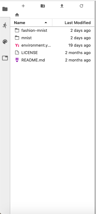
The left sidebar can be collapsed or expanded by selecting “Show Left Sidebar” in the View menu or by clicking on the active sidebar tab.
Main Work Area
The main work area in JupyterLab enables you to arrange documents (notebooks, text files, etc.) and other activities (terminals, code consoles, etc.) into panels of tabs that can be resized or subdivided. A screenshot of the default Menu Bar is provided below.
Drag a tab to the center of a tab panel to move the tab to the panel. Subdivide a tab panel by dragging a tab to the left, right, top, or bottom of the panel. The work area has a single current activity. The tab for the current activity is marked with a colored top border (blue by default).
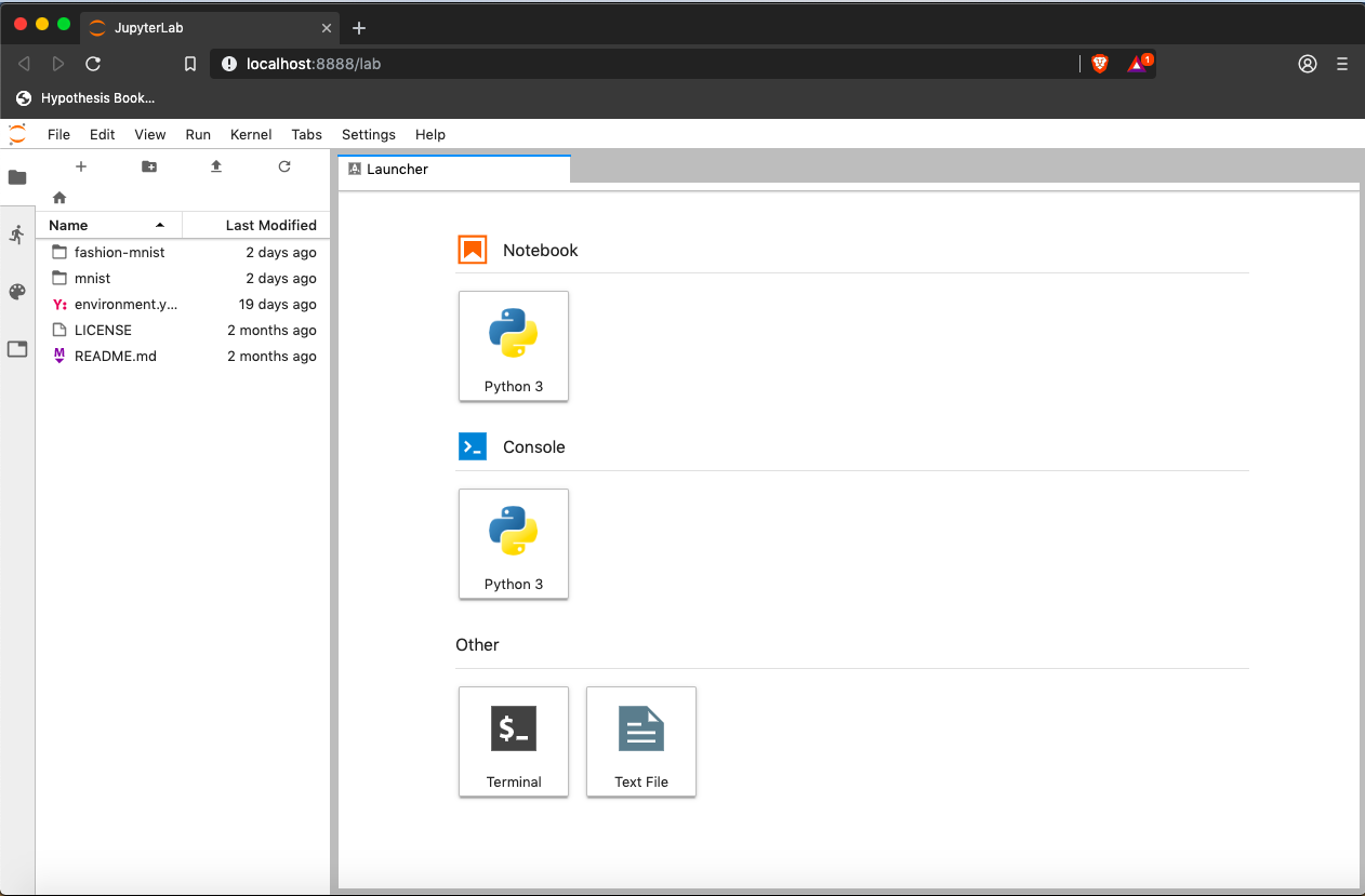
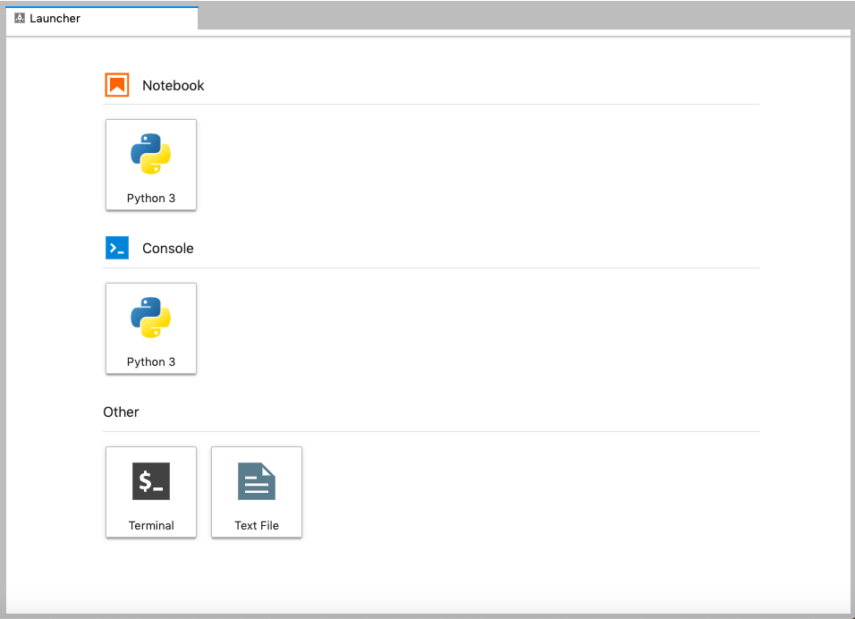
Creating a Python script
- To start writing a new Python program click the Text File icon under the Other header in the Launcher tab of the Main Work Area.
- You can also create a new plain text file by selecting the New -> Text File from the File menu in the Menu Bar.
- To convert this plain text file to a Python program, select the Save File As action from the File menu in the Menu Bar and give your new text file a name that ends with the
.pyextension.- The
.pyextension lets everyone (including the operating system) know that this text file is a Python program. - This is convention, not a requirement.
- The
Creating a Jupyter Notebook
To open a new notebook click the Python 3 icon under the Notebook header in the Launcher tab in the main work area. You can also create a new notebook by selecting New -> Notebook from the File menu in the Menu Bar.
Additional notes on Jupyter notebooks.
- Notebook files have the extension
.ipynbto distinguish them from plain-text Python programs. - Notebooks can be exported as Python scripts that can be run from the command line.
Below is a screenshot of a Jupyter notebook running inside JupyterLab. If you are interested in more details, then see the official notebook documentation.
How It’s Stored
- The notebook file is stored in a format called JSON.
- Just like a webpage, what’s saved looks different from what you see in your browser.
- But this format allows Jupyter to mix source code, text, and images, all in one file.
Arranging Documents into Panels of Tabs
In the JupyterLab Main Work Area you can arrange documents into panels of tabs. Here is an example from the official documentation.
First, create a text file, Python console, and terminal window and arrange them into three panels in the main work area. Next, create a notebook, terminal window, and text file and arrange them into three panels in the main work area. Finally, create your own combination of panels and tabs. What combination of panels and tabs do you think will be most useful for your workflow?
Solution
After creating the necessary tabs, you can drag one of the tabs to the center of a panel to move the tab to the panel; next you can subdivide a tab panel by dragging a tab to the left, right, top, or bottom of the panel.
Use the Jupyter Notebook for editing and running Python.
- While it’s common to write Python scripts using a text editor, we are going to use the Jupyter Notebook for the remainder of this workshop.
- This has several advantages:
- You can easily type, edit, and copy and paste blocks of code.
- Tab complete allows you to easily access the names of things you are using and learn more about them.
- It allows you to annotate your code with links, different sized text, bullets, etc. to make it more accessible to you and your collaborators.
- It allows you to display figures next to the code that produces them to tell a complete story of the analysis.
- Each notebook contains one or more cells that contain code, text, or images.
Code vs. Text
Jupyter mixes code and text in different types of blocks, called cells. We often use the term “code” to mean “the source code of software written in a language such as Python”. A “code cell” in a Notebook is a cell that contains software; a “text cell” is one that contains ordinary prose written for human beings.
The Notebook has Command and Edit modes.
- If you press Esc and Return alternately, the outer border of your code cell will change from gray to blue.
- These are the Command (gray) and Edit (blue) modes of your notebook.
- Command mode allows you to edit notebook-level features, and Edit mode changes the content of cells.
- When in Command mode (esc/gray),
- The b key will make a new cell below the currently selected cell.
- The a key will make one above.
- The x key will delete the current cell.
- The z key will undo your last cell operation (which could be a deletion, creation, etc).
- All actions can be done using the menus, but there are lots of keyboard shortcuts to speed things up.
Command Vs. Edit
In the Jupyter notebook page are you currently in Command or Edit mode?
Switch between the modes. Use the shortcuts to generate a new cell. Use the shortcuts to delete a cell. Use the shortcuts to undo the last cell operation you performed.Solution
Command mode has a grey border and Edit mode has a blue border. Use Esc and Return to switch between modes. You need to be in Command mode (Press Esc if your cell is blue). Type b or a. You need to be in Command mode (Press Esc if your cell is blue). Type x. You need to be in Command mode (Press Esc if your cell is blue). Type z.
Use the keyboard and mouse to select and edit cells.
- Pressing the Return key turns the border blue and engages Edit mode, which allows you to type within the cell.
- Because we want to be able to write many lines of code in a single cell, pressing the Return key when in Edit mode (blue) moves the cursor to the next line in the cell just like in a text editor.
- We need some other way to tell the Notebook we want to run what’s in the cell.
- Pressing Shift+Return together will execute the contents of the cell.
- Notice that the Return and Shift keys on the right of the keyboard are right next to each other.
The Notebook will turn Markdown into pretty-printed documentation.
- Notebooks can also render Markdown.
- A simple plain-text format for writing lists, links, and other things that might go into a web page.
- Equivalently, a subset of HTML that looks like what you’d send in an old-fashioned email.
- Turn the current cell into a Markdown cell by entering the Command mode (Esc/gray) and press the M key.
In [ ]:will disappear to show it is no longer a code cell and you will be able to write in Markdown.- Markdown cells have to be executed similar to Python cells with Shift+Return.
- Turn the current cell into a Code cell by entering the Command mode (Esc/gray) and press the y key.
Markdown does most of what HTML does.
*   Use asterisks
*   to create
*   bullet lists.
- Use asterisks
- to create
- bullet lists.
1.  Use numbers
1.  to create
1.  numbered lists.
- Use numbers
- to create
- numbered lists.
*  You can use indents
	*  To create sublists
	*  of the same type
*  Or sublists
	1. Of different
	1. types
- You can use indents
- To create sublists
- of the same type
- Or sublists
- Of different
- types
# A Level-1 Heading
A Level-1 Heading
## A Level-2 Heading (etc.)
A Level-2 Heading (etc.)
Line breaks
don't matter.

But blank lines
create new paragraphs.
Line breaks don’t matter.
But blank lines create new paragraphs.
[Create links](http://software-carpentry.org) with `[...](...)`.
Or use [named links][data_carpentry].

[data_carpentry]: http://datacarpentry.org
Create links with [...](...).
Or use named links.
Creating Lists in Markdown
Create a nested list in a Markdown cell in a notebook that looks like this:
- Get funding.
- Do work.
- Design experiment.
- Collect data.
- Analyze.
- Write up.
- Publish.
Solution
This challenge integrates both the numbered list and bullet list. Note that the bullet list is indented 2 spaces so that it is inline with the items of the numbered list.
1.  Get funding.
2.  Do work.
    *   Design experiment.
    *   Collect data.
    *   Analyze.
3.  Write up.
4.  Publish.
More Math
What is displayed when a Python cell in a notebook that contains several calculations is executed? For example, what happens when this cell is executed?
7 * 3
2 + 1
Solution
Python returns the output of the last calculation.
3
Change an Existing Cell from Code to Markdown
What happens if you write some Python in a code cell and then you switch it to a Markdown cell? For example, put the following in a code cell:
x = 6 * 7 + 12
print(x)
And then run it with Shift+Return to be sure that it works as a code cell. Now go back to the cell and use Esc then m to switch the cell to Markdown and “run” it with Shift+Return. What happened and how might this be useful?
Solution
The Python code gets treated like Markdown text. The lines appear as if they are part of one contiguous paragraph. This could be useful to temporarily turn on and off cells in notebooks that get used for multiple purposes.
x = 6 * 7 + 12 print(x)
Equations
Standard Markdown (such as we’re using for these notes) won’t render equations, but the Notebook will. Create a new Markdown cell and enter the following:
$\sum_{i=1}^{N} 2^{-i} \approx 1$(It’s probably easier to copy and paste.) What does it display? What do you think the underscore,
_, circumflex,^, and dollar sign,$, do?Solution
The notebook shows the equation as it would be rendered from LaTeX equation syntax. The dollar sign,
$, is used to tell Markdown that the text in between is a LaTeX equation. If you’re not familiar with LaTeX, underscore,_, is used for subscripts and circumflex,^, is used for superscripts. A pair of curly braces,{and}, is used to group text together so that the statementi=1becomes the subscript andNbecomes the superscript. Similarly,-iis in curly braces to make the whole statement the superscript for2.\sumand\approxare LaTeX commands for “sum over” and “approximate” symbols.
Closing JupyterLab
- From the Menu Bar select the “File” menu and the choose “Shut Down” at the bottom of the dropdown menu. You will be prompted to confirm that you wish to shutdown the JupyterLab server (don’t forget to save your work!). Click “Shut Down” to shutdown the JupyterLab server.
- To restart the JupyterLab server you will need to re-run the following command from a shell.
$ jupyter lab
Closing JupyerLab
Practice closing and restarting the JupyterLab server.
Key Points
Python scripts are plain text files.
Use the Jupyter Notebook for editing and running Python.
The Notebook has Command and Edit modes.
Use the keyboard and mouse to select and edit cells.
The Notebook will turn Markdown into pretty-printed documentation.
Markdown does most of what HTML does.
Python Fundamentals
Overview
Teaching: 20 min
Exercises: 10 minQuestions
What basic data types can I work with in Python?
How can I create a new variable in Python?
Can I change the value associated with a variable after I create it?
Objectives
Assign values to variables.
Variables
Any Python interpreter can be used as a calculator:
3 + 5 * 4
23
This is great but not very interesting.
To do anything useful with data, we need to assign its value to a variable.
In Python, we can assign a value to a
variable, using the equals sign =.
For example, to assign value 60 to a variable weight_kg, we would execute:
weight_kg = 60
From now on, whenever we use weight_kg, Python will substitute the value we assigned to
it. In layman’s terms, a variable is a name for a value.
In Python, variable names:
- can include letters, digits, and underscores
- cannot start with a digit
- are case sensitive.
This means that, for example:
weight0is a valid variable name, whereas0weightis notweightandWeightare different variables
Introducing types of data
Python knows various types of data. Three common ones are:
- integer numbers
- floating point numbers, and
- strings.
In the example above, variable weight_kg has an integer value of 60.
To create a variable with a floating point value, we can execute:
weight_kg = 60.0
And to create a string, we add single or double quotes around some text, for example:
weight_kg_text = 'weight in kilograms:'
Using Variables in Python
To display the value of a variable to the screen in Python, we can use the print function:
print(weight_kg)
60.0
We can display multiple things at once using only one print command:
print(weight_kg_text, weight_kg)
weight in kilograms: 60.0
Moreover, we can do arithmetic with variables right inside the print function:
print('weight in pounds:', 2.2 * weight_kg)
weight in pounds: 132.0
The above command, however, did not change the value of weight_kg:
print(weight_kg)
60.0
To change the value of the weight_kg variable, we have to
assign weight_kg a new value using the equals = sign:
weight_kg = 65.0
print('weight in kilograms is now:', weight_kg)
weight in kilograms is now: 65.0
Variables as Sticky Notes
A variable is analogous to a sticky note with a name written on it: assigning a value to a variable is like putting that sticky note on a particular value.
This means that assigning a value to one variable does not change values of other variables. For example, let’s store the subject’s weight in pounds in its own variable:
# There are 2.2 pounds per kilogram
weight_lb = 2.2 * weight_kg
print(weight_kg_text, weight_kg, 'and in pounds:', weight_lb)
weight in kilograms: 65.0 and in pounds: 143.0
Let’s now change
weight_kg:weight_kg = 100.0 print('weight in kilograms is now:', weight_kg, 'and weight in pounds is still:', weight_lb)weight in kilograms is now: 100.0 and weight in pounds is still: 143.0
Since
weight_lbdoesn’t “remember” where its value comes from, it is not updated when we changeweight_kg.


Use meaningful variable names.
- Python doesn’t care what you call variables as long as they obey the rules (alphanumeric characters and the underscore).
var1 = 42
ewr_422_yY = 'Ahmed'
print(ewr_422_yY, 'is', var1, 'years old')
- Use meaningful variable names to help other people understand what the program does.
- The most important “other person” is your future self.
- Python itself proposes a standard style including variable naming style through one of its first Python Enhancement Proposals (PEP), PEP8.
Check Your Understanding
What values do the variables
massandagehave after each statement in the following program? Test your answers by executing the commands.mass = 47.5 age = 122 mass = mass * 2.0 age = age - 20 print(mass, age)Solution
95.0 102
Sorting Out References
What does the following program print out?
first, second = 'Grace', 'Hopper'
third, fourth = second, first
print(third, fourth)
Solution
Hopper Grace
Key Points
Basic data types in Python include integers, strings, and floating-point numbers.
Use
variable = valueto assign a value to a variable in order to record it in memory.Variables are created on demand whenever a value is assigned to them.
Use
print(something)to display the value ofsomething.
Data Types and Type Conversion
Overview
Teaching: 20 min
Exercises: 10 minQuestions
What kinds of data do programs store?
How can I convert one type to another?
Objectives
Explain key differences between integers and floating point numbers.
Explain key differences between numbers and character strings.
Perform some operations using strings.
Use built-in functions to convert between integers, floating point numbers, and strings.
Every value has a type.
- Every value in a program has a specific type.
- Integer (
int): represents positive or negative whole numbers like 3 or -512. - Floating point number (
float): represents real numbers like 3.14159 or -2.5. - Character string (usually called “string”,
str): text.- Written in either single quotes or double quotes (as long as they match).
- The quote marks aren’t printed when the string is displayed.
Use the built-in function type to find the type of a value.
- Use the built-in function
typeto find out what type a value has. - Works on variables as well.
- But remember: the value has the type — the variable is just a label.
print(type(52))
<class 'int'>
fitness = 'average'
print(type(fitness))
<class 'str'>
Types control what operations (or methods) can be performed on a given value.
- A value’s type determines what the program can do to it.
print(5 - 3)
2
print('hello' - 'h')
---------------------------------------------------------------------------
TypeError                                 Traceback (most recent call last)
<ipython-input-2-67f5626a1e07> in <module>()
----> 1 print('hello' - 'h')

TypeError: unsupported operand type(s) for -: 'str' and 'str'
You can use the “+” and “*” operators on strings.
- “Adding” character strings concatenates them.
full_name = 'Ahmed' + ' ' + 'Walsh'
print(full_name)
Ahmed Walsh
- Multiplying a character string by an integer N creates a new string that consists of that character string repeated N times.
- Since multiplication is repeated addition.
separator = '=' * 10
print(separator)
==========
Strings have a length (but numbers don’t).
- The built-in function
lencounts the number of characters in a string.
print(len(full_name))
11
- But numbers don’t have a length (not even zero).
print(len(52))
---------------------------------------------------------------------------
TypeError                                 Traceback (most recent call last)
<ipython-input-3-f769e8e8097d> in <module>()
----> 1 print(len(52))

TypeError: object of type 'int' has no len()
We must convert numbers to strings or vice versa when operating on them.
- Cannot add numbers and strings.
print(1 + '2')
---------------------------------------------------------------------------
TypeError                                 Traceback (most recent call last)
<ipython-input-4-fe4f54a023c6> in <module>()
----> 1 print(1 + '2')

TypeError: unsupported operand type(s) for +: 'int' and 'str'
- Not allowed because it’s ambiguous: should
1 + '2'be3or'12'? - Some types can be converted to other types by using the type name as a function.
print(1 + int('2'))
print(str(1) + '2')
3
12
More operations on strings
- We can operate on strings with specialized functions (there are many more):
a = 'space alpacas'
a.title()
a.upper()
a.startswith('b')
a.isdigit()
'Space Alpacas'
'SPACE ALPACAS'
False
False
Inserting variables into strings
- The older, clunkier approach is to use %-formatting:
name = 'Anna'
age = 24
'Hello, %s. You are %s.' % (name, age)"
'Hello Anna. You are 24.'
- The
%sterms tell the interpreter to insert - as strings - the values in brackets (variables in this case) after the%following the main string. - %-formatting becomes hard to follow when many variables need to be inserted.
- We can use f-strings for a more elegant approach:
name = 'Anna'
age = 24
f'Hello, {name}. You are {age}.'
'Hello Anna. You are 24.'
Escape sequences
- For including a newline or tab in a string we can use the escape sequences,
\nand\trespectively.
We can mix integers and floats freely in operations.
- Integers and floating-point numbers can be mixed in arithmetic.
- Python 3 automatically converts integers to floats as needed. (Integer division in Python 2 will return an integer, the floor of the division.)
print('half is', 1 / 2.0)
print('three squared is', 3.0 ** 2)
half is 0.5
three squared is 9.0
Variables only change value when something is assigned to them.
- If we make one cell in a spreadsheet depend on another, and update the latter, the former updates automatically.
- This does not happen in programming languages.
first = 1
second = 5 * first
first = 2
print('first is', first, 'and second is', second)
first is 2 and second is 5
- The computer reads the value of
firstwhen doing the multiplication, creates a new value, and assigns it tosecond. - After that,
seconddoes not remember where it came from.
Fractions
What type of value is 3.4? How can you find out?
Solution
It is a floating-point number (often abbreviated “float”).
print(type(3.4))<class 'float'>
Automatic Type Conversion
What type of value is 3.25 + 4?
Solution
It is a float: integers are automatically converted to floats as necessary.
result = 3.25 + 4
print(result, 'is', type(result))
7.25 is <class 'float'>
Choose a Type
What type of value (integer, floating point number, or character string) would you use to represent each of the following? Try to come up with more than one good answer for each problem. For example, in # 1, when would counting days with a floating point variable make more sense than using an integer?
- Number of days since the start of the year.
- Time elapsed from the start of the year until now in days.
- Serial number of a piece of lab equipment.
- A lab specimen’s age
- Current population of a city.
- Average population of a city over time.
Solution
The answers to the questions are:
- Integer, since the number of days would lie between 1 and 365.
- Floating point, since fractional days are required
- Character string if serial number contains letters and numbers, otherwise integer if the serial number consists only of numerals
- This will vary! How do you define a specimen’s age? whole days since collection (integer)? date and time (string)?
- Choose floating point to represent population as large aggregates (eg millions), or integer to represent population in units of individuals.
- Floating point number, since an average is likely to have a fractional part.
Division Types
In Python 3, the
//operator performs integer (whole-number) floor division, the/operator performs floating-point division, and the ‘%’ (or modulo) operator calculates and returns the remainder from integer division:print('5 // 3:', 5//3) print('5 / 3:', 5/3) print('5 % 3:', 5%3)5 // 3: 1 5 / 3: 1.6666666666666667 5 % 3: 2However in Python2 (and other languages), the
/operator between two integer types perform a floor (//) division. To perform a float division, we have to convert one of the integers to float.print('5 // 3:', 1) print('5 / 3:', 1 ) print('5 / float(3):', 1.6666667 ) print('float(5) / 3:', 1.6666667 ) print('float(5 / 3):', 1.0 ) print('5 % 3:', 2)If
num_subjectsis the number of subjects taking part in a study, andnum_per_surveyis the number that can take part in a single survey, write an expression that calculates the number of surveys needed to reach everyone once.Solution
We want the minimum number of surveys that reaches everyone once, which is the rounded up value of
num_subjects / num_per_survey. This is equivalent to performing an integer division with//and adding 1.num_subjects = 600 num_per_survey = 42 num_surveys = num_subjects // num_per_survey + 1 print(num_subjects, 'subjects,', num_per_survey, 'per survey:', num_surveys)600 subjects, 42 per survey: 15
Strings to Numbers
Where reasonable,
float()will convert a string to a floating point number, andint()will convert a floating point number to an integer:print("string to float:", float("3.4")) print("float to int:", int(3.4))string to float: 3.4 float to int: 3If the conversion doesn’t make sense, however, an error message will occur
print("string to float:", float("Hello world!"))--------------------------------------------------------------------------- ValueError Traceback (most recent call last) <ipython-input-5-df3b790bf0a2> in <module>() ----> 1 print("string to float:", float("Hello world!")) ValueError: could not convert string to float: 'Hello world!'Given this information, what do you expect the following program to do?
What does it actually do?
Why do you think it does that?
print("fractional string to int:", int("3.4"))Solution
What do you expect this program to do? It would not be so unreasonable to expect the Python 3
intcommand to convert the string “3.4” to 3.4 and an additional type conversion to 3. After all, Python 3 performs a lot of other magic - isn’t that part of its charm?However, Python 3 throws an error. Why? To be consistent, possibly. If you ask Python to perform two consecutive typecasts, you must convert it explicitly in code.
int("3.4")
int(float("3.4"))
In [2]: int("3.4") --------------------------------------------------------------------------- ValueError Traceback (most recent call last) <ipython-input-2-ec6729dfccdc> in <module>() ----> 1 int("3.4") ValueError: invalid literal for int() with base 10: '3.4' 3
Arithmetic with Different Types
Which of the following will return the floating point number
2.0? Note: there may be more than one right answer.first = 1.0 second = "1" third = "1.1"
first + float(second)float(second) + float(third)first + int(third)first + int(float(third))int(first) + int(float(third))2.0 * secondSolution
Answer: 1 and 4
Complex Numbers
Python provides complex numbers, which are written as
1.0+2.0j. Ifvalis a complex number, its real and imaginary parts can be accessed using dot notation asval.realandval.imag.complex = 6 + 2j print(complex.real) print(complex.imag)6.0 2.0
- Why do you think Python uses
jinstead ofifor the imaginary part?- What do you expect
1+2j + 3to produce?- What do you expect
4jto be? What about4 jor4 + j?Solution
- Standard mathematics treatments typically use
ito denote an imaginary number. However, from media reports it was an early convention established from electrical engineering that now presents a technically expensive area to change. Stack Overflow provides additional explanation and discussion.(4+2j)4j,Syntax Error: invalid syntax, in this case j is considered a variable and this depends on if j is defined and if so, its assigned value
Key Points
Every value has a type.
Use the built-in function
typeto find the type of a value.Types control what operations can be done on values.
Strings can be added and multiplied.
Strings have a length (but numbers don’t).
Strings can be elegantly built up from variables by using f-string formatting.
Must convert numbers to strings or vice versa when operating on them.
Can mix integers and floats freely in operations.
Variables only change value when something is assigned to them.
Libraries
Overview
Teaching: 10 min
Exercises: 10 minQuestions
How can I use software that other people have written?
How can I find out what that software does?
Objectives
Explain what software libraries are and why programmers create and use them.
Write programs that import and use modules from Python’s standard library.
Find and read documentation for the standard library interactively (in the interpreter) and online.
Most of the power of a programming language is in its libraries.
- A library is a collection of files (called modules) that contains
functions for use by other programs.
- May also contain data values (e.g., numerical constants) and other things.
- Library’s contents are supposed to be related, but there’s no way to enforce that.
- The Python standard library is an extensive suite of modules that comes with Python itself.
- Many additional libraries are available from PyPI (the Python Package Index).
- We will see later how to write new libraries.
Libraries and modules
A library is a collection of modules, but the terms are often used interchangeably, especially since many libraries only consist of a single module, so don’t worry if you mix them.
A program must import a library module before using it.
- Use
importto load a library module into a program’s memory. - Then refer to things from the module as
module_name.thing_name.- Python uses
.to mean “part of”.
- Python uses
- Using
math, one of the modules in the standard library:
import math

print('pi is', math.pi)
print('cos(pi) is', math.cos(math.pi))
pi is 3.141592653589793
cos(pi) is -1.0
- Have to refer to each item with the module’s name.
math.cos(pi)won’t work: the reference topidoesn’t somehow “inherit” the function’s reference tomath.
Use help to learn about the contents of a library module.
- Works just like help for a function.
help(math)
Help on module math:

NAME
    math

MODULE REFERENCE
    http://docs.python.org/3/library/math

    The following documentation is automatically generated from the Python
    source files.  It may be incomplete, incorrect or include features that
    are considered implementation detail and may vary between Python
    implementations.  When in doubt, consult the module reference at the
    location listed above.

DESCRIPTION
    This module is always available.  It provides access to the
    mathematical functions defined by the C standard.

FUNCTIONS
    acos(x, /)
        Return the arc cosine (measured in radians) of x.
⋮ ⋮ ⋮
Import specific items from a library module to shorten programs.
- Use
from ... import ...to load only specific items from a library module. - Then refer to them directly without library name as prefix.
from math import cos, pi

print('cos(pi) is', cos(pi))
cos(pi) is -1.0
However, you must be careful here, because of name clashes with functions imported from other libraries with the same name, e.g. numpy.cos. To avoid this problem, we recommend avoiding importing specific items - use aliases to shorten instead.
Create an alias for a library module when importing it to shorten programs.
- Use
import ... as ...to give a library a short alias while importing it. - Then refer to items in the library using that shortened name.
import math as m

print('cos(pi) is', m.cos(m.pi))
cos(pi) is -1.0
- Commonly used for libraries that are frequently used or have long names.
- E.g., the
matplotlibplotting library is often aliased asmpl.
- E.g., the
- But can make programs harder to understand, since readers must learn your program’s aliases.
Exploring the Math Module
- What function from the
mathmodule can you use to calculate a square root without usingsqrt?- Since the library contains this function, why does
sqrtexist?Solution
- Using
help(math)we see that we’ve gotpow(x,y)in addition tosqrt(x), so we could usepow(x, 0.5)to find a square root.The
sqrt(x)function is arguably more readable thanpow(x, 0.5)when implementing equations. Readability is a cornerstone of good programming, so it makes sense to provide a special function for this specific common case.Also, the design of Python’s
mathlibrary has its origin in the C standard, which includes bothsqrt(x)andpow(x,y), so a little bit of the history of programming is showing in Python’s function names.
Locating the Right Module
You want to select a random character from a string:
bases = 'ACTTGCTTGAC'
- Which standard library module could help you?
- Which function would you select from that module? Are there alternatives?
- Try to write a program that uses the function.
Solution
The random module seems like it could help you.
The string has 11 characters, each having a positional index from 0 to 10. You could use
random.randrangefunction (or the aliasrandom.randintif you find that easier to remember) to get a random integer between 0 and 10, and then pick out the character at that position:from random import randrange random_index = randrange(len(bases)) print(bases[random_index])or more compactly:
from random import randrange

print(bases[randrange(len(bases))])
Perhaps you found the
random.samplefunction? It allows for slightly less typing:from random import sample print(sample(bases, 1)[0])Note that this function returns a list of values. We will learn about lists in episode 11.
There’s also other functions you could use, but with more convoluted code as a result.
Jigsaw Puzzle (Parson’s Problem) Programming Example
Rearrange the following statements so that a random DNA base is printed and its index in the string. Not all statements may be needed. Feel free to use/add intermediate variables.
bases="ACTTGCTTGAC"
import math
import random
___ = random.randrange(n_bases)
___ = len(bases)
print("random base ", bases[___], "base index", ___)
Solution
import math
import random
bases = "ACTTGCTTGAC"
n_bases = len(bases)
idx = random.randrange(n_bases)
print("random base", bases[idx], "base index", idx)
When Is Help Available?
When a colleague of yours types
help(math), Python reports an error:NameError: name 'math' is not definedWhat has your colleague forgotten to do?
Solution
Importing the math module (
import math)
Importing With Aliases
- Fill in the blanks so that the program below prints
90.0.- Rewrite the program so that it uses
importwithoutas.- Which form do you find easier to read?
import math as m
angle = ____.degrees(____.pi / 2)
print(____)
Solution
import math as m
angle = m.degrees(m.pi / 2)
print(angle)
can be written as
import math
angle = math.degrees(math.pi / 2)
print(angle)
Since you just wrote the code and are familiar with it, you might actually find the first version easier to read. But when trying to read a huge piece of code written by someone else, or when getting back to your own huge piece of code after several months, non-abbreviated names are often easier, except where there are clear abbreviation conventions.
There Are Many Ways To Import Libraries!
Match the following print statements with the appropriate library calls.
Print commands:
print("sin(pi/2) =", sin(pi/2))print("sin(pi/2) =", m.sin(m.pi/2))print("sin(pi/2) =", math.sin(math.pi/2))Library calls:
from math import sin, piimport mathimport math as mfrom math import *Solution
- Library calls 1 and 4. In order to directly refer to
sinandpiwithout the library name as prefix, you need to use thefrom ... import ...statement. Whereas library call 1 specifically imports the two functionssinandpi, library call 4 imports all functions in themathmodule.- Library call 3. Here
sinandpiare referred to with a shortened library nameminstead ofmath. Library call 3 does exactly that using theimport ... as ...syntax - it creates an alias formathin the form of the shortened namem.- Library call 2. Here
sinandpiare referred to with the regular library namemath, so the regularimport ...call suffices.
Importing Specific Items
- Fill in the blanks so that the program below prints
90.0.- Do you find this version easier to read than preceding ones?
- Why wouldn’t programmers always use this form of
import?____ math import ____, ____ angle = degrees(pi / 2) print(angle)Solution
from math import degrees, pi
angle = degrees(pi / 2)
print(angle)
Most likely you find this version easier to read since it’s less dense. The main reason not to use this form of import is to avoid name clashes. For instance, you wouldn’t import
degreesthis way if you also wanted to use the namedegreesfor a variable or function of your own. Or if you were to also import a function nameddegreesfrom another library.
Reading Error Messages
- Read the code below and try to identify what the errors are without running it.
- Run the code, and read the error message. What type of error is it?
from math import log
log(0)
Solution
- The logarithm of
xis only defined forx > 0, so 0 is outside the domain of the function.- You get an error of type “ValueError”, indicating that the function received an inappropriate argument value. The additional message “math domain error” makes it clearer what the problem is.
Key Points
Most of the power of a programming language is in its libraries.
A program must import a library module in order to use it.
Use
helpto learn about the contents of a library module.Import specific items from a library to shorten programs.
Create an alias for a library when importing it to shorten programs.
Analyzing Patient Data
Overview
Teaching: 40 min
Exercises: 20 minQuestions
How can I process tabular data files in Python?
Objectives
Explain what a library is and what libraries are used for.
Import a Python library and use the functions it contains.
Read tabular data from a file into a program.
Select individual values and subsections from data.
Perform operations on arrays of data.
Words are useful, but what’s more useful are the sentences and stories we build with them. Similarly, while a lot of powerful, general tools are built into Python, specialized tools built up from these basic units live in libraries that can be called upon when needed.
Loading data into Python
To begin processing inflammation data, we need to load it into Python. We can do that using a library called NumPy, which stands for Numerical Python. In general, you should use this library when you want to do fancy things with lots of numbers, especially if you have matrices or arrays. To tell Python that we’d like to start using NumPy, we need to import it:
import numpy
Importing a library is like getting a piece of lab equipment out of a storage locker and setting it up on the bench. Libraries provide additional functionality to the basic Python package, much like a new piece of equipment adds functionality to a lab space. Just like in the lab, importing too many libraries can sometimes complicate and slow down your programs - so we only import what we need for each program.
Once we’ve imported the library, we can ask the library to read our data file for us:
numpy.loadtxt(fname='inflammation-01.csv', delimiter=',')
array([[ 0.,  0.,  1., ...,  3.,  0.,  0.],
       [ 0.,  1.,  2., ...,  1.,  0.,  1.],
       [ 0.,  1.,  1., ...,  2.,  1.,  1.],
       ...,
       [ 0.,  1.,  1., ...,  1.,  1.,  1.],
       [ 0.,  0.,  0., ...,  0.,  2.,  0.],
       [ 0.,  0.,  1., ...,  1.,  1.,  0.]])
The expression numpy.loadtxt(...) is a function call
that asks Python to run the function loadtxt which
belongs to the numpy library. This dotted notation
is used everywhere in Python: the thing that appears before the dot contains the thing that
appears after.
As an example, John Smith is the John that belongs to the Smith family.
We could use the dot notation to write his name smith.john,
just as loadtxt is a function that belongs to the numpy library.
numpy.loadtxt has two parameters: the name of the file
we want to read and the delimiter that separates values on
a line. These both need to be character strings (or strings
for short), so we put them in quotes.
Since we haven’t told it to do anything else with the function’s output,
the notebook displays it.
In this case,
that output is the data we just loaded.
By default,
only a few rows and columns are shown
(with ... to omit elements when displaying big arrays).
Note that, to save space when displaying NumPy arrays, Python does not show us trailing zeros, so 1.0 becomes 1..
Importing libraries with shortcuts
In this lesson we use the
import numpysyntax to import NumPy. However, shortcuts such asimport numpy as npare frequently used. Importing NumPy this way means that after the inital import, rather than writingnumpy.loadtxt(...), you can now writenp.loadtxt(...). Some people prefer this as it is quicker to type and results in shorter lines of code - especially for libraries with long names! You will frequently see Python code online using a NumPy function withnp, and it’s because they’ve used this shortcut. It makes no difference which approach you choose to take, but you must be consistent as if you useimport numpy as npthennumpy.loadtxt(...)will not work, and you must usenp.loadtxt(...)instead. Because of this, when working with other people it is important you agree on how libraries are imported.
Our call to numpy.loadtxt read our file
but didn’t save the data in memory.
To do that,
we need to assign the array to a variable. In a similar manner to how we assign a single
value to a variable, we can also assign an array of values to a variable using the same syntax.
Let’s re-run numpy.loadtxt and save the returned data:
data = numpy.loadtxt(fname='inflammation-01.csv', delimiter=',')
This statement doesn’t produce any output because we’ve assigned the output to the variable data.
If we want to check that the data have been loaded,
we can print the variable’s value:
print(data)
[[ 0.  0.  1. ...,  3.  0.  0.]
 [ 0.  1.  2. ...,  1.  0.  1.]
 [ 0.  1.  1. ...,  2.  1.  1.]
 ...,
 [ 0.  1.  1. ...,  1.  1.  1.]
 [ 0.  0.  0. ...,  0.  2.  0.]
 [ 0.  0.  1. ...,  1.  1.  0.]]
Now that the data are in memory,
we can manipulate them.
First,
let’s ask what type of thing data refers to:
print(type(data))
<class 'numpy.ndarray'>
The output tells us that data currently refers to
an N-dimensional array, the functionality for which is provided by the NumPy library.
These data correspond to arthritis patients’ inflammation.
The rows are the individual patients, and the columns
are their daily inflammation measurements.
Data Type
A Numpy array contains one or more elements of the same type. The
typefunction will only tell you that a variable is a NumPy array but won’t tell you the type of thing inside the array. We can find out the type of the data contained in the NumPy array.print(data.dtype)float64This tells us that the NumPy array’s elements are floating-point numbers.
With the following command, we can see the array’s shape:
print(data.shape)
(60, 40)
The output tells us that the data array variable contains 60 rows and 40 columns. When we
created the variable data to store our arthritis data, we did not only create the array; we also
created information about the array, called members or
attributes. This extra information describes data in the same way an adjective describes a noun.
data.shape is an attribute of data which describes the dimensions of data. We use the same
dotted notation for the attributes of variables that we use for the functions in libraries because
they have the same part-and-whole relationship.
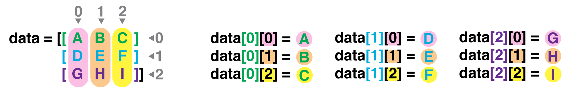
If we want to get a single number from the array, we must provide an index in square brackets after the variable name, just as we do in math when referring to an element of a matrix. Our inflammation data has two dimensions, so we will need to use two indices to refer to one specific value:
print('first value in data:', data[0, 0])
first value in data: 0.0
print('middle value in data:', data[30, 20])
middle value in data: 13.0
The expression data[30, 20] accesses the element at row 30, column 20. While this expression may
not surprise you,
data[0, 0] might.
Programming languages like Fortran, MATLAB and R start counting at 1
because that’s what human beings have done for thousands of years.
Languages in the C family (including C++, Java, Perl, and Python) count from 0
because it represents an offset from the first value in the array (the second
value is offset by one index from the first value). This is closer to the way
that computers represent arrays (if you are interested in the historical
reasons behind counting indices from zero, you can read
Mike Hoye’s blog post).
As a result,
if we have an M×N array in Python,
its indices go from 0 to M-1 on the first axis
and 0 to N-1 on the second.
It takes a bit of getting used to,
but one way to remember the rule is that
the index is how many steps we have to take from the start to get the item we want.
In the Corner
What may also surprise you is that when Python displays an array, it shows the element with index
[0, 0]in the upper left corner rather than the lower left. This is consistent with the way mathematicians draw matrices but different from the Cartesian coordinates. The indices are (row, column) instead of (column, row) for the same reason, which can be confusing when plotting data.
Slicing data
An index like [30, 20] selects a single element of an array,
but we can select whole sections as well.
For example,
we can select the first ten days (columns) of values
for the first four patients (rows) like this:
print(data[0:4, 0:10])
[[ 0.  0.  1.  3.  1.  2.  4.  7.  8.  3.]
 [ 0.  1.  2.  1.  2.  1.  3.  2.  2.  6.]
 [ 0.  1.  1.  3.  3.  2.  6.  2.  5.  9.]
 [ 0.  0.  2.  0.  4.  2.  2.  1.  6.  7.]]
The slice 0:4 means, “Start at index 0 and go up to, but not
including, index 4”. Again, the up-to-but-not-including takes a bit of getting used to, but the
rule is that the difference between the upper and lower bounds is the number of values in the slice.
We don’t have to start slices at 0:
print(data[5:10, 0:10])
[[ 0.  0.  1.  2.  2.  4.  2.  1.  6.  4.]
 [ 0.  0.  2.  2.  4.  2.  2.  5.  5.  8.]
 [ 0.  0.  1.  2.  3.  1.  2.  3.  5.  3.]
 [ 0.  0.  0.  3.  1.  5.  6.  5.  5.  8.]
 [ 0.  1.  1.  2.  1.  3.  5.  3.  5.  8.]]
We also don’t have to include the upper and lower bound on the slice. If we don’t include the lower bound, Python uses 0 by default; if we don’t include the upper, the slice runs to the end of the axis, and if we don’t include either (i.e., if we use ‘:’ on its own), the slice includes everything:
small = data[:3, 36:]
print('small is:')
print(small)
The above example selects rows 0 through 2 and columns 36 through to the end of the array.
small is:
[[ 2.  3.  0.  0.]
 [ 1.  1.  0.  1.]
 [ 2.  2.  1.  1.]]
Analyzing data
NumPy has several useful functions that take an array as input to perform operations on its values.
If we want to find the average inflammation for all patients on
all days, for example, we can ask NumPy to compute data’s mean value:
print(numpy.mean(data))
6.14875
mean is a function that takes
an array as an argument.
Not All Functions Have Input
Generally, a function uses inputs to produce outputs. However, some functions produce outputs without needing any input. For example, checking the current time doesn’t require any input.
import time
print(time.ctime())
Sat Mar 26 13:07:33 2016For functions that don’t take in any arguments, we still need parentheses (
()) to tell Python to go and do something for us.
Let’s use three other NumPy functions to get some descriptive values about the dataset. We’ll also use multiple assignment, a convenient Python feature that will enable us to do this all in one line.
maxval, minval, stdval = numpy.max(data), numpy.min(data), numpy.std(data)

print('maximum inflammation:', maxval)
print('minimum inflammation:', minval)
print('standard deviation:', stdval)
Here we’ve assigned the return value from numpy.max(data) to the variable maxval, the value
from numpy.min(data) to minval, and so on.
maximum inflammation: 20.0
minimum inflammation: 0.0
standard deviation: 4.61383319712
Mystery Functions in IPython
How did we know what functions NumPy has and how to use them? If you are working in IPython or in a Jupyter Notebook, there is an easy way to find out. If you type the name of something followed by a dot, then you can use tab completion (e.g. type
numpy.and then press Tab) to see a list of all functions and attributes that you can use. After selecting one, you can also add a question mark (e.g.numpy.cumprod?), and IPython will return an explanation of the method! This is the same as doinghelp(numpy.cumprod). Similarly, if you are using the “plain vanilla” Python interpreter, you can typenumpy.and press the Tab key twice for a listing of what is available. You can then use thehelp()function to see an explanation of the function you’re interested in, for example:help(numpy.cumprod).
When analyzing data, though, we often want to look at variations in statistical values, such as the maximum inflammation per patient or the average inflammation per day. One way to do this is to create a new temporary array of the data we want, then ask it to do the calculation:
patient_0 = data[0, :] # 0 on the first axis (rows), everything on the second (columns)
print('maximum inflammation for patient 0:', numpy.max(patient_0))
maximum inflammation for patient 0: 18.0
Everything in a line of code following the ‘#’ symbol is a comment that is ignored by Python. Comments allow programmers to leave explanatory notes for other programmers or their future selves.
We don’t actually need to store the row in a variable of its own. Instead, we can combine the selection and the function call:
print('maximum inflammation for patient 2:', numpy.max(data[2, :]))
maximum inflammation for patient 2: 19.0
What if we need the maximum inflammation for each patient over all days (as in the next diagram on the left) or the average for each day (as in the diagram on the right)? As the diagram below shows, we want to perform the operation across an axis:
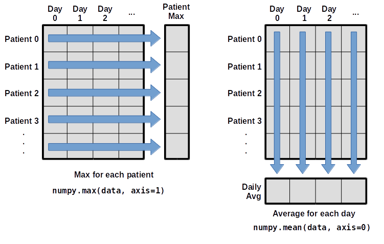
To support this functionality, most array functions allow us to specify the axis we want to work on. If we ask for the average across axis 0 (rows in our 2D example), we get:
print(numpy.mean(data, axis=0))
[  0.           0.45         1.11666667   1.75         2.43333333   3.15
   3.8          3.88333333   5.23333333   5.51666667   5.95         5.9
   8.35         7.73333333   8.36666667   9.5          9.58333333
  10.63333333  11.56666667  12.35        13.25        11.96666667
  11.03333333  10.16666667  10.           8.66666667   9.15         7.25
   7.33333333   6.58333333   6.06666667   5.95         5.11666667   3.6
   3.3          3.56666667   2.48333333   1.5          1.13333333
   0.56666667]
As a quick check, we can ask this array what its shape is:
print(numpy.mean(data, axis=0).shape)
(40,)
The expression (40,) tells us we have an N×1 vector,
so this is the average inflammation per day for all patients.
If we average across axis 1 (columns in our 2D example), we get:
print(numpy.mean(data, axis=1))
[ 5.45   5.425  6.1    5.9    5.55   6.225  5.975  6.65   6.625  6.525
  6.775  5.8    6.225  5.75   5.225  6.3    6.55   5.7    5.85   6.55
  5.775  5.825  6.175  6.1    5.8    6.425  6.05   6.025  6.175  6.55
  6.175  6.35   6.725  6.125  7.075  5.725  5.925  6.15   6.075  5.75
  5.975  5.725  6.3    5.9    6.75   5.925  7.225  6.15   5.95   6.275  5.7
  6.1    6.825  5.975  6.725  5.7    6.25   6.4    7.05   5.9  ]
which is the average inflammation per patient across all days.
Slicing Strings
A section of an array is called a slice. We can take slices of character strings as well:
element = 'oxygen'
print('first three characters:', element[0:3])
print('last three characters:', element[3:6])
first three characters: oxy last three characters: genWhat is the value of
element[:4]? What aboutelement[4:]? Orelement[:]?Solution
oxyg
en
oxygen
What is
element[-1]? What iselement[-2]?Solution
n
e
Given those answers, explain what
element[1:-1]does.Solution
Creates a substring from index 1 up to (not including) the final index, effectively removing the first and last letters from ‘oxygen’
How can we rewrite the slice for getting the last three characters of
element, so that it works even if we assign a different string toelement? Test your solution with the following strings:carpentry,clone,hi.Solution
element = 'oxygen'
print('last three characters:', element[-3:])
element = 'carpentry'
print('last three characters:', element[-3:])
element = 'clone'
print('last three characters:', element[-3:])
element = 'hi'
print('last three characters:', element[-3:])
last three characters: gen last three characters: try last three characters: one last three characters: hi
Thin Slices
The expression
element[3:3]produces an empty string, i.e., a string that contains no characters. Ifdataholds our array of patient data, what doesdata[3:3, 4:4]produce? What aboutdata[3:3, :]?Solution
array([], shape=(0, 0), dtype=float64)
array([], shape=(0, 40), dtype=float64)
Stacking Arrays
Arrays can be concatenated and stacked on top of one another, using NumPy’s
vstackandhstackfunctions for vertical and horizontal stacking, respectively.import numpy A = numpy.array([[1,2,3], [4,5,6], [7, 8, 9]]) print('A = ') print(A) B = numpy.hstack([A, A]) print('B = ') print(B) C = numpy.vstack([A, A]) print('C = ') print(C)A = [[1 2 3] [4 5 6] [7 8 9]] B = [[1 2 3 1 2 3] [4 5 6 4 5 6] [7 8 9 7 8 9]] C = [[1 2 3] [4 5 6] [7 8 9] [1 2 3] [4 5 6] [7 8 9]]Write some additional code that slices the first and last columns of
A, and stacks them into a 3x2 array. Make sure toSolution
A ‘gotcha’ with array indexing is that singleton dimensions are dropped by default. That means
A[:, 0]is a one dimensional array, which won’t stack as desired. To preserve singleton dimensions, the index itself can be a slice or array. For example,A[:, :1]returns a two dimensional array with one singleton dimension (i.e. a column vector).D = numpy.hstack((A[:, :1], A[:, -1:])) print('D = ') print(D)D = [[1 3] [4 6] [7 9]]Solution
An alternative way to achieve the same result is to use Numpy’s delete function to remove the second column of A.
D = numpy.delete(A, 1, 1)
print('D = ')
print(D)
D = [[1 3] [4 6] [7 9]]
Change In Inflammation
The patient data is longitudinal in the sense that each row represents a series of observations relating to one individual. This means that the change in inflammation over time is a meaningful concept. Let’s find out how to calculate changes in the data contained in an array with NumPy.
The
numpy.diff()function takes an array and returns the differences between two successive values. Let’s use it to examine the changes each day across the first week of patient 3 from our inflammation dataset.patient3_week1 = data[3, :7] print(patient3_week1)[0. 0. 2. 0. 4. 2. 2.]Calling
numpy.diff(patient3_week1)would do the following calculations[ 0 - 0, 2 - 0, 0 - 2, 4 - 0, 2 - 4, 2 - 2 ]and return the 6 difference values in a new array.
numpy.diff(patient3_week1)array([ 0., 2., -2., 4., -2., 0.])Note that the array of differences is shorter by one element (length 6).
When calling
numpy.diffwith a multi-dimensional array, anaxisargument may be passed to the function to specify which axis to process. When applyingnumpy.diffto our 2D inflammation arraydata, which axis would we specify?Solution
Since the row axis (0) is patients, it does not make sense to get the difference between two arbitrary patients. The column axis (1) is in days, so the difference is the change in inflammation – a meaningful concept.
numpy.diff(data, axis=1)If the shape of an individual data file is
(60, 40)(60 rows and 40 columns), what would the shape of the array be after you run thediff()function and why?Solution
The shape will be
(60, 39)because there is one fewer difference between columns than there are columns in the data.How would you find the largest change in inflammation for each patient? Does it matter if the change in inflammation is an increase or a decrease?
Solution
By using the
numpy.max()function after you apply thenumpy.diff()function, you will get the largest difference between days.numpy.max(numpy.diff(data, axis=1), axis=1)array([ 7., 12., 11., 10., 11., 13., 10., 8., 10., 10., 7., 7., 13., 7., 10., 10., 8., 10., 9., 10., 13., 7., 12., 9., 12., 11., 10., 10., 7., 10., 11., 10., 8., 11., 12., 10., 9., 10., 13., 10., 7., 7., 10., 13., 12., 8., 8., 10., 10., 9., 8., 13., 10., 7., 10., 8., 12., 10., 7., 12.])If inflammation values decrease along an axis, then the difference from one element to the next will be negative. If you are interested in the magnitude of the change and not the direction, the
numpy.absolute()function will provide that.Notice the difference if you get the largest absolute difference between readings.
numpy.max(numpy.absolute(numpy.diff(data, axis=1)), axis=1)array([ 12., 14., 11., 13., 11., 13., 10., 12., 10., 10., 10., 12., 13., 10., 11., 10., 12., 13., 9., 10., 13., 9., 12., 9., 12., 11., 10., 13., 9., 13., 11., 11., 8., 11., 12., 13., 9., 10., 13., 11., 11., 13., 11., 13., 13., 10., 9., 10., 10., 9., 9., 13., 10., 9., 10., 11., 13., 10., 10., 12.])
Key Points
Import a library into a program using
import libraryname.Use the
numpylibrary to work with arrays in Python.The expression
array.shapegives the shape of an array.Use
array[x, y]to select a single element from a 2D array.Array indices start at 0, not 1.
Use
low:highto specify aslicethat includes the indices fromlowtohigh-1.Use
# some kind of explanationto add comments to programs.Use
numpy.mean(array),numpy.max(array), andnumpy.min(array)to calculate simple statistics.Use
numpy.mean(array, axis=0)ornumpy.mean(array, axis=1)to calculate statistics across the specified axis.
Visualizing Tabular Data
Overview
Teaching: 30 min
Exercises: 20 minQuestions
How can I visualize tabular data in Python?
How can I group several plots together?
Objectives
Plot simple graphs from data.
Group several graphs in a single figure.
Visualizing data
The mathematician Richard Hamming once said, “The purpose of computing is insight, not numbers,” and
the best way to develop insight is often to visualize data. Visualization deserves an entire
lecture of its own, but we can explore a few features of Python’s matplotlib library here. While
there is no official plotting library, matplotlib is the de facto standard. First, we will
import the pyplot module from matplotlib and use two of its functions to create and display a
heat map of our data:
import matplotlib.pyplot
image = matplotlib.pyplot.imshow(data)
matplotlib.pyplot.show()

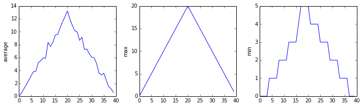
Blue pixels in this heat map represent low values, while yellow pixels represent high values. As we can see, inflammation rises and falls over a 40-day period. Let’s take a look at the average inflammation over time:
ave_inflammation = numpy.mean(data, axis=0)
ave_plot = matplotlib.pyplot.plot(ave_inflammation)
matplotlib.pyplot.show()

Here, we have put the average inflammation per day across all patients in the variable ave_inflammation, then
asked matplotlib.pyplot to create and display a line graph of those values. The result is a
roughly linear rise and fall, which is suspicious: we might instead expect a sharper rise and slower
fall. Let’s have a look at two other statistics:
max_plot = matplotlib.pyplot.plot(numpy.max(data, axis=0))
matplotlib.pyplot.show()

min_plot = matplotlib.pyplot.plot(numpy.min(data, axis=0))
matplotlib.pyplot.show()

The maximum value rises and falls smoothly, while the minimum seems to be a step function. Neither trend seems particularly likely, so either there’s a mistake in our calculations or something is wrong with our data. This insight would have been difficult to reach by examining the numbers themselves without visualization tools.
Grouping plots
You can group similar plots in a single figure using subplots.
This script below uses a number of new commands. The function matplotlib.pyplot.figure()
creates a space into which we will place all of our plots. The parameter figsize
tells Python how big to make this space. Each subplot is placed into the figure using
its add_subplot method. The add_subplot method takes 3
parameters. The first denotes how many total rows of subplots there are, the second parameter
refers to the total number of subplot columns, and the final parameter denotes which subplot
your variable is referencing (left-to-right, top-to-bottom). Each subplot is stored in a
different variable (axes1, axes2, axes3). Once a subplot is created, the axes can
be titled using the set_xlabel() command (or set_ylabel()).
Here are our three plots side by side:
import numpy
import matplotlib.pyplot

data = numpy.loadtxt(fname='inflammation-01.csv', delimiter=',')

fig = matplotlib.pyplot.figure(figsize=(10.0, 3.0))

axes1 = fig.add_subplot(1, 3, 1)
axes2 = fig.add_subplot(1, 3, 2)
axes3 = fig.add_subplot(1, 3, 3)

axes1.set_ylabel('average')
axes1.plot(numpy.mean(data, axis=0))

axes2.set_ylabel('max')
axes2.plot(numpy.max(data, axis=0))

axes3.set_ylabel('min')
axes3.plot(numpy.min(data, axis=0))

fig.tight_layout()

matplotlib.pyplot.savefig('inflammation.png')
matplotlib.pyplot.show()

The call to loadtxt reads our data,
and the rest of the program tells the plotting library
how large we want the figure to be,
that we’re creating three subplots,
what to draw for each one,
and that we want a tight layout.
(If we leave out that call to fig.tight_layout(),
the graphs will actually be squeezed together more closely.)
The call to savefig stores the plot as a graphics file. This can be
a convenient way to store your plots for use in other documents, web
pages etc. The graphics format is automatically determined by
Matplotlib from the file name ending we specify; here PNG from
‘inflammation.png’. Matplotlib supports many different graphics
formats, including SVG, PDF, and JPEG.
Plot Scaling
Why do all of our plots stop just short of the upper end of our graph?
Solution
Because matplotlib normally sets x and y axes limits to the min and max of our data (depending on data range)
If we want to change this, we can use the
set_ylim(min, max)method of each ‘axes’, for example:axes3.set_ylim(0,6)Update your plotting code to automatically set a more appropriate scale. (Hint: you can make use of the
maxandminmethods to help.)Solution
# One method
axes3.set_ylabel('min')
axes3.plot(numpy.min(data, axis=0))
axes3.set_ylim(0,6)
Solution
# A more automated approach
min_data = numpy.min(data, axis=0)
axes3.set_ylabel('min')
axes3.plot(min_data)
axes3.set_ylim(numpy.min(min_data), numpy.max(min_data) * 1.1)
Drawing Straight Lines
In the center and right subplots above, we expect all lines to look like step functions because non-integer value are not realistic for the minimum and maximum values. However, you can see that the lines are not always vertical or horizontal, and in particular the step function in the subplot on the right looks slanted. Why is this?
Solution
Because matplotlib interpolates (draws a straight line) between the points. One way to do avoid this is to use the Matplotlib
drawstyleoption:import numpy import matplotlib.pyplot data = numpy.loadtxt(fname='inflammation-01.csv', delimiter=',') fig = matplotlib.pyplot.figure(figsize=(10.0, 3.0)) axes1 = fig.add_subplot(1, 3, 1) axes2 = fig.add_subplot(1, 3, 2) axes3 = fig.add_subplot(1, 3, 3) axes1.set_ylabel('average') axes1.plot(numpy.mean(data, axis=0), drawstyle='steps-mid') axes2.set_ylabel('max') axes2.plot(numpy.max(data, axis=0), drawstyle='steps-mid') axes3.set_ylabel('min') axes3.plot(numpy.min(data, axis=0), drawstyle='steps-mid') fig.tight_layout() matplotlib.pyplot.show()

Make Your Own Plot
Create a plot showing the standard deviation (
numpy.std) of the inflammation data for each day across all patients.Solution
std_plot = matplotlib.pyplot.plot(numpy.std(data, axis=0))
matplotlib.pyplot.show()
Moving Plots Around
Modify the program to display the three plots on top of one another instead of side by side.
Solution
import numpy
import matplotlib.pyplot

data = numpy.loadtxt(fname='inflammation-01.csv', delimiter=',')

# change figsize (swap width and height)
fig = matplotlib.pyplot.figure(figsize=(3.0, 10.0))

# change add_subplot (swap first two parameters)
axes1 = fig.add_subplot(3, 1, 1)
axes2 = fig.add_subplot(3, 1, 2)
axes3 = fig.add_subplot(3, 1, 3)

axes1.set_ylabel('average')
axes1.plot(numpy.mean(data, axis=0))

axes2.set_ylabel('max')
axes2.plot(numpy.max(data, axis=0))

axes3.set_ylabel('min')
axes3.plot(numpy.min(data, axis=0))

fig.tight_layout()

matplotlib.pyplot.show()
Key Points
Use the
pyplotmodule from thematplotliblibrary for creating simple visualizations.
Repeating Actions with Loops
Overview
Teaching: 30 min
Exercises: 0 minQuestions
How can I do the same operations on many different values?
Objectives
Explain what a
forloop does.Correctly write
forloops to repeat simple calculations.Trace changes to a loop variable as the loop runs.
Trace changes to other variables as they are updated by a
forloop.
In the last episode, we wrote Python code that plots values of interest from our first
inflammation dataset (inflammation-01.csv), which revealed some suspicious features in it.
We have a dozen data sets right now, though, and more on the way. We want to create plots for all of our data sets with a single statement. To do that, we’ll have to teach the computer how to repeat things.
An example task that we might want to repeat is printing each character in a word on a line of its own.
word = 'lead'
In Python, a string is basically an ordered collection of characters, and every
character has a unique number associated with it – its index. This means that
we can access characters in a string using their indices.
For example, we can get the first character of the word 'lead', by using
word[0]. One way to print each character is to use four print statements:
print(word[0])
print(word[1])
print(word[2])
print(word[3])
l
e
a
d
This is a bad approach for three reasons:
-
Not scalable. Imagine you need to print characters of a string that is hundreds of letters long. It might be easier to type them in manually.
-
Difficult to maintain. If we want to decorate each printed character with an asterisk or any other character, we would have to change four lines of code. While this might not be a problem for short strings, it would definitely be a problem for longer ones.
-
Fragile. If we use it with a word that has more characters than what we initially envisioned, it will only display part of the word’s characters. A shorter string, on the other hand, will cause an error because it will be trying to display part of the string that doesn’t exist.
word = 'tin'
print(word[0])
print(word[1])
print(word[2])
print(word[3])
t
i
n
---------------------------------------------------------------------------
IndexError                                Traceback (most recent call last)
<ipython-input-3-7974b6cdaf14> in <module>()
      3 print(word[1])
      4 print(word[2])
----> 5 print(word[3])

IndexError: string index out of range
Here’s a better approach:
word = 'lead'
for char in word:
    print(char)
l
e
a
d
This is shorter — certainly shorter than something that prints every character in a hundred-letter string — and more robust as well:
word = 'oxygen'
for char in word:
    print(char)
o
x
y
g
e
n
The improved version uses a for loop to repeat an operation — in this case, printing — once for each thing in a sequence. The general form of a loop is:
for variable in collection:
    # do things using variable, such as print
Using the oxygen example above, the loop might look like this:
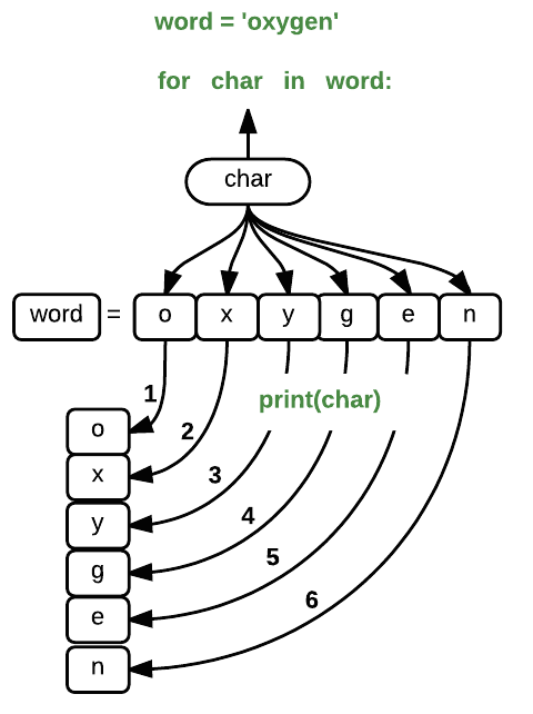
where each character (char) in the variable word is looped through and printed one character
after another. The numbers in the diagram denote which loop cycle the character was printed in (1
being the first loop, and 6 being the final loop).
We can call the loop variable anything we like, but
there must be a colon at the end of the line starting the loop, and we must indent anything we
want to run inside the loop. Unlike many other languages, there is no command to signify the end
of the loop body (e.g. end for); what is indented after the for statement belongs to the loop.
What’s in a name?
In the example above, the loop variable was given the name
charas a mnemonic; it is short for ‘character’. We can choose any name we want for variables. We can even call our loop variablebanana, as long as we use this name consistently:word = 'oxygen' for banana in word: print(banana)o x y g e nIt is a good idea to choose variable names that are meaningful, otherwise it would be more difficult to understand what the loop is doing.
Here’s another loop that repeatedly updates a variable:
length = 0
for vowel in 'aeiou':
    length = length + 1
print('There are', length, 'vowels')
There are 5 vowels
It’s worth tracing the execution of this little program step by step.
Since there are five characters in 'aeiou',
the statement on line 3 will be executed five times.
The first time around,
length is zero (the value assigned to it on line 1)
and vowel is 'a'.
The statement adds 1 to the old value of length,
producing 1,
and updates length to refer to that new value.
The next time around,
vowel is 'e' and length is 1,
so length is updated to be 2.
After three more updates,
length is 5;
since there is nothing left in 'aeiou' for Python to process,
the loop finishes
and the print statement on line 4 tells us our final answer.
Note that a loop variable is a variable that’s being used to record progress in a loop. It still exists after the loop is over, and we can re-use variables previously defined as loop variables as well:
letter = 'z'
for letter in 'abc':
    print(letter)
print('after the loop, letter is', letter)
a
b
c
after the loop, letter is c
Note also that finding the length of a string is such a common operation
that Python actually has a built-in function to do it called len:
print(len('aeiou'))
5
len is much faster than any function we could write ourselves,
and much easier to read than a two-line loop;
it will also give us the length of many other things that we haven’t met yet,
so we should always use it when we can.
From 1 to N
Python has a built-in function called
rangethat generates a sequence of numbers.rangecan accept 1, 2, or 3 parameters.
- If one parameter is given,
rangegenerates a sequence of that length, starting at zero and incrementing by 1. For example,range(3)produces the numbers0, 1, 2.- If two parameters are given,
rangestarts at the first and ends just before the second, incrementing by one. For example,range(2, 5)produces2, 3, 4.- If
rangeis given 3 parameters, it starts at the first one, ends just before the second one, and increments by the third one. For example,range(3, 10, 2)produces3, 5, 7, 9.Using
range, write a loop that usesrangeto print the first 3 natural numbers:1 2 3Solution
for number in range(1, 4): print(number)
Understanding the loops
Given the following loop:
word = 'oxygen' for char in word: print(char)How many times is the body of the loop executed?
- 3 times
- 4 times
- 5 times
- 6 times
Solution
The body of the loop is executed 6 times.
Computing Powers With Loops
Exponentiation is built into Python:
print(5 ** 3)125Write a loop that calculates the same result as
5 ** 3using multiplication (and without exponentiation).Solution
result = 1 for number in range(0, 3): result = result * 5 print(result)
Reverse a String
Knowing that two strings can be concatenated using the
+operator, write a loop that takes a string and produces a new string with the characters in reverse order, so'Newton'becomes'notweN'.Solution
newstring = '' oldstring = 'Newton' for char in oldstring: newstring = char + newstring print(newstring)
Computing the Value of a Polynomial
The built-in function
enumeratetakes a sequence (e.g. a list) and generates a new sequence of the same length. Each element of the new sequence is a pair composed of the index (0, 1, 2,…) and the value from the original sequence:for idx, val in enumerate(a_list): # Do something using idx and valThe code above loops through
a_list, assigning the index toidxand the value toval.Suppose you have encoded a polynomial as a list of coefficients in the following way: the first element is the constant term, the second element is the coefficient of the linear term, the third is the coefficient of the quadratic term, etc.
x = 5 coefs = [2, 4, 3] y = coefs[0] * x**0 + coefs[1] * x**1 + coefs[2] * x**2 print(y)97Write a loop using
enumerate(coefs)which computes the valueyof any polynomial, givenxandcoefs.Solution
y = 0 for idx, coef in enumerate(coefs): y = y + coef * x**idx
Key Points
Use
for variable in sequenceto process the elements of a sequence one at a time.The body of a
forloop must be indented.Use
len(thing)to determine the length of something that contains other values.
Storing Multiple Values in Lists
Overview
Teaching: 30 min
Exercises: 15 minQuestions
How can I store many values together?
Objectives
Explain what a list is.
Create and index lists of simple values.
Change the values of individual elements
Append values to an existing list
Reorder and slice list elements
Create and manipulate nested lists
Similar to a string that can contain many characters, a list is a container that can store many values. Unlike NumPy arrays, lists are built into the language (so we don’t have to load a library to use them). We create a list by putting values inside square brackets and separating the values with commas:
odds = [1, 3, 5, 7]
print('odds are:', odds)
odds are: [1, 3, 5, 7]
We can access elements of a list using indices – numbered positions of elements in the list. These positions are numbered starting at 0, so the first element has an index of 0.
print('first element:', odds[0])
print('last element:', odds[3])
print('"-1" element:', odds[-1])
first element: 1
last element: 7
"-1" element: 7
Yes, we can use negative numbers as indices in Python. When we do so, the index -1 gives us the
last element in the list, -2 the second to last, and so on.
Because of this, odds[3] and odds[-1] point to the same element here.
If we loop over a list, the loop variable is assigned to its elements one at a time:
for number in odds:
print(number)
1
3
5
7
There is one important difference between lists and strings: we can change the values in a list, but we cannot change individual characters in a string. For example:
names = ['Curie', 'Darwing', 'Turing'] # typo in Darwin's name
print('names is originally:', names)
names[1] = 'Darwin' # correct the name
print('final value of names:', names)
names is originally: ['Curie', 'Darwing', 'Turing']
final value of names: ['Curie', 'Darwin', 'Turing']
works, but:
name = 'Darwin'
name[0] = 'd'
---------------------------------------------------------------------------
TypeError Traceback (most recent call last)
<ipython-input-8-220df48aeb2e> in <module>()
1 name = 'Darwin'
----> 2 name[0] = 'd'
TypeError: 'str' object does not support item assignment
does not.
Ch-Ch-Ch-Ch-Changes
Data which can be modified in place is called mutable, while data which cannot be modified is called immutable. Strings and numbers are immutable. This does not mean that variables with string or number values are constants, but when we want to change the value of a string or number variable, we can only replace the old value with a completely new value.
Lists and arrays, on the other hand, are mutable: we can modify them after they have been created. We can change individual elements, append new elements, or reorder the whole list. For some operations, like sorting, we can choose whether to use a function that modifies the data in-place or a function that returns a modified copy and leaves the original unchanged.
Be careful when modifying data in-place. If two variables refer to the same list, and you modify the list value, it will change for both variables!
salsa = ['peppers', 'onions', 'cilantro', 'tomatoes'] my_salsa = salsa # <-- my_salsa and salsa point to the *same* list data in memory salsa[0] = 'hot peppers' print('Ingredients in my salsa:', my_salsa)Ingredients in my salsa: ['hot peppers', 'onions', 'cilantro', 'tomatoes']If you want variables with mutable values to be independent, you must make a copy of the value when you assign it.
salsa = ['peppers', 'onions', 'cilantro', 'tomatoes'] my_salsa = list(salsa) # <-- makes a *copy* of the list salsa[0] = 'hot peppers' print('Ingredients in my salsa:', my_salsa)Ingredients in my salsa: ['peppers', 'onions', 'cilantro', 'tomatoes']Because of pitfalls like this, code which modifies data in place can be more difficult to understand. However, it is often far more efficient to modify a large data structure in place than to create a modified copy for every small change. You should consider both of these aspects when writing your code.
Nested Lists
Since a list can contain any Python variables, it can even contain other lists.
For example, we could represent the products in the shelves of a small grocery shop:
x = [['pepper', 'zucchini', 'onion'], ['cabbage', 'lettuce', 'garlic'], ['apple', 'pear', 'banana']]Here is a visual example of how indexing a list of lists
xworks:
Using the previously declared list
x, these would be the results of the index operations shown in the image:print([x[0]])[['pepper', 'zucchini', 'onion']]print(x[0])['pepper', 'zucchini', 'onion']print(x[0][0])'pepper'Thanks to Hadley Wickham for the image above.
![x is represented as a pepper shaker containing several packets of pepper. [x[0]] is represented
as a pepper shaker containing a single packet of pepper. x[0] is represented as a single packet of
pepper. x[0][0] is represented as single grain of pepper. Adapted
from @hadleywickham.](../fig/indexing_lists_python.png)
Heterogeneous Lists
Lists in Python can contain elements of different types. Example:
sample_ages = [10, 12.5, 'Unknown']
There are many ways to change the contents of lists besides assigning new values to individual elements:
odds.append(11)
print('odds after adding a value:', odds)
odds after adding a value: [1, 3, 5, 7, 11]
removed_element = odds.pop(0)
print('odds after removing the first element:', odds)
print('removed_element:', removed_element)
odds after removing the first element: [3, 5, 7, 11]
removed_element: 1
odds.reverse()
print('odds after reversing:', odds)
odds after reversing: [11, 7, 5, 3]
While modifying in place, it is useful to remember that Python treats lists in a slightly counter-intuitive way.
As we saw earlier, when we modified the salsa list item in-place, if we make a list, (attempt to) copy it and then modify this list, we can cause all sorts of trouble. This also applies to modifying the list using the above functions:
odds = [1, 3, 5, 7]
primes = odds
primes.append(2)
print('primes:', primes)
print('odds:', odds)
primes: [1, 3, 5, 7, 2]
odds: [1, 3, 5, 7, 2]
This is because Python stores a list in memory, and then can use multiple names to refer to the
same list. If all we want to do is copy a (simple) list, we can again use the list function, so we do
not modify a list we did not mean to:
odds = [1, 3, 5, 7]
primes = list(odds)
primes.append(2)
print('primes:', primes)
print('odds:', odds)
primes: [1, 3, 5, 7, 2]
odds: [1, 3, 5, 7]
Turn a String Into a List
Use a for-loop to convert the string “hello” into a list of letters:
['h', 'e', 'l', 'l', 'o']Hint: You can create an empty list like this:
my_list = []Solution
my_list = [] for char in 'hello': my_list.append(char) print(my_list)
Subsets of lists and strings can be accessed by specifying ranges of values in brackets, similar to how we accessed ranges of positions in a NumPy array. This is commonly referred to as “slicing” the list/string.
binomial_name = 'Drosophila melanogaster'
group = binomial_name[0:10]
print('group:', group)
species = binomial_name[11:23]
print('species:', species)
chromosomes = ['X', 'Y', '2', '3', '4']
autosomes = chromosomes[2:5]
print('autosomes:', autosomes)
last = chromosomes[-1]
print('last:', last)
group: Drosophila
species: melanogaster
autosomes: ['2', '3', '4']
last: 4
Slicing From the End
Use slicing to access only the last four characters of a string or entries of a list.
string_for_slicing = 'Observation date: 02-Feb-2013' list_for_slicing = [['fluorine', 'F'], ['chlorine', 'Cl'], ['bromine', 'Br'], ['iodine', 'I'], ['astatine', 'At']]'2013' [['chlorine', 'Cl'], ['bromine', 'Br'], ['iodine', 'I'], ['astatine', 'At']]Would your solution work regardless of whether you knew beforehand the length of the string or list (e.g. if you wanted to apply the solution to a set of lists of different lengths)? If not, try to change your approach to make it more robust.
Hint: Remember that indices can be negative as well as positive
Solution
Use negative indices to count elements from the end of a container (such as list or string):
string_for_slicing[-4:] list_for_slicing[-4:]
Non-Continuous Slices
So far we’ve seen how to use slicing to take single blocks of successive entries from a sequence. But what if we want to take a subset of entries that aren’t next to each other in the sequence?
You can achieve this by providing a third argument to the range within the brackets, called the step size. The example below shows how you can take every third entry in a list:
primes = [2, 3, 5, 7, 11, 13, 17, 19, 23, 29, 31, 37] subset = primes[0:12:3] print('subset', subset)subset [2, 7, 17, 29]Notice that the slice taken begins with the first entry in the range, followed by entries taken at equally-spaced intervals (the steps) thereafter. If you wanted to begin the subset with the third entry, you would need to specify that as the starting point of the sliced range:
primes = [2, 3, 5, 7, 11, 13, 17, 19, 23, 29, 31, 37] subset = primes[2:12:3] print('subset', subset)subset [5, 13, 23, 37]Use the step size argument to create a new string that contains only every other character in the string “In an octopus’s garden in the shade”. Start with creating a variable to hold the string:
beatles = "In an octopus's garden in the shade"What slice of
beatleswill produce the following output (i.e., the first character, third character, and every other character through the end of the string)?I notpssgre ntesaeSolution
To obtain every other character you need to provide a slice with the step size of 2:
beatles[0:35:2]You can also leave out the beginning and end of the slice to take the whole string and provide only the step argument to go every second element:
beatles[::2]
If you want to take a slice from the beginning of a sequence, you can omit the first index in the range:
date = 'Monday 4 January 2016'
day = date[0:6]
print('Using 0 to begin range:', day)
day = date[:6]
print('Omitting beginning index:', day)
Using 0 to begin range: Monday
Omitting beginning index: Monday
And similarly, you can omit the ending index in the range to take a slice to the very end of the sequence:
months = ['jan', 'feb', 'mar', 'apr', 'may', 'jun', 'jul', 'aug', 'sep', 'oct', 'nov', 'dec']
sond = months[8:12]
print('With known last position:', sond)
sond = months[8:len(months)]
print('Using len() to get last entry:', sond)
sond = months[8:]
print('Omitting ending index:', sond)
With known last position: ['sep', 'oct', 'nov', 'dec']
Using len() to get last entry: ['sep', 'oct', 'nov', 'dec']
Omitting ending index: ['sep', 'oct', 'nov', 'dec']
Overloading
+usually means addition, but when used on strings or lists, it means “concatenate”. Given that, what do you think the multiplication operator*does on lists? In particular, what will be the output of the following code?counts = [2, 4, 6, 8, 10] repeats = counts * 2 print(repeats)
[2, 4, 6, 8, 10, 2, 4, 6, 8, 10][4, 8, 12, 16, 20][[2, 4, 6, 8, 10],[2, 4, 6, 8, 10]][2, 4, 6, 8, 10, 4, 8, 12, 16, 20]The technical term for this is operator overloading: a single operator, like
+or*, can do different things depending on what it’s applied to.Solution
The multiplication operator
*used on a list replicates elements of the list and concatenates them together:[2, 4, 6, 8, 10, 2, 4, 6, 8, 10]It’s equivalent to:
counts + counts
Key Points
[value1, value2, value3, ...]creates a list.Lists can contain any Python object, including lists (i.e., list of lists).
Lists are indexed and sliced with square brackets (e.g., list[0] and list[2:9]), in the same way as strings and arrays.
Lists are mutable (i.e., their values can be changed in place).
Strings are immutable (i.e., the characters in them cannot be changed).
Analyzing Data from Multiple Files
Overview
Teaching: 20 min
Exercises: 0 minQuestions
How can I do the same operations on many different files?
Objectives
Use a library function to get a list of filenames that match a wildcard pattern.
Write a
forloop to process multiple files.
We now have almost everything we need to process all our data files. The only thing that’s missing is a library with a rather unpleasant name:
import glob
The glob library contains a function, also called glob,
that finds files and directories whose names match a pattern.
We provide those patterns as strings:
the character * matches zero or more characters,
while ? matches any one character.
We can use this to get the names of all the CSV files in the current directory:
print(glob.glob('inflammation*.csv'))
['inflammation-05.csv', 'inflammation-11.csv', 'inflammation-12.csv', 'inflammation-08.csv',
'inflammation-03.csv', 'inflammation-06.csv', 'inflammation-09.csv', 'inflammation-07.csv',
'inflammation-10.csv', 'inflammation-02.csv', 'inflammation-04.csv', 'inflammation-01.csv']
As these examples show,
glob.glob’s result is a list of file and directory paths in arbitrary order.
This means we can loop over it
to do something with each filename in turn.
In our case,
the “something” we want to do is generate a set of plots for each file in our inflammation dataset.
If we want to start by analyzing just the first three files in alphabetical order, we can use the
sorted built-in function to generate a new sorted list from the glob.glob output:
import glob
import numpy
import matplotlib.pyplot
filenames = sorted(glob.glob('inflammation*.csv'))
filenames = filenames[0:3]
for filename in filenames:
print(filename)
data = numpy.loadtxt(fname=filename, delimiter=',')
fig = matplotlib.pyplot.figure(figsize=(10.0, 3.0))
axes1 = fig.add_subplot(1, 3, 1)
axes2 = fig.add_subplot(1, 3, 2)
axes3 = fig.add_subplot(1, 3, 3)
axes1.set_ylabel('average')
axes1.plot(numpy.mean(data, axis=0))
axes2.set_ylabel('max')
axes2.plot(numpy.max(data, axis=0))
axes3.set_ylabel('min')
axes3.plot(numpy.min(data, axis=0))
fig.tight_layout()
matplotlib.pyplot.show()
inflammation-01.csv

inflammation-02.csv
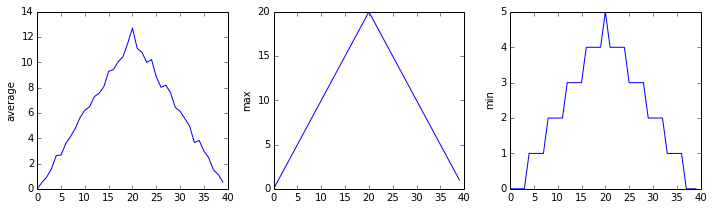
inflammation-03.csv
Sure enough, the maxima of the first two data sets show exactly the same ramp as the first, and their minima show the same staircase structure; a different situation has been revealed in the third dataset, where the maxima are a bit less regular, but the minima are consistently zero.
Plotting Differences
Plot the difference between the average inflammations reported in the first and second datasets (stored in
inflammation-01.csvandinflammation-02.csv, correspondingly), i.e., the difference between the leftmost plots of the first two figures.Solution
import glob import numpy import matplotlib.pyplot filenames = sorted(glob.glob('inflammation*.csv')) data0 = numpy.loadtxt(fname=filenames[0], delimiter=',') data1 = numpy.loadtxt(fname=filenames[1], delimiter=',') fig = matplotlib.pyplot.figure(figsize=(10.0, 3.0)) matplotlib.pyplot.ylabel('Difference in average') matplotlib.pyplot.plot(numpy.mean(data0, axis=0) - numpy.mean(data1, axis=0)) fig.tight_layout() matplotlib.pyplot.show()
Generate Composite Statistics
Use each of the files once to generate a dataset containing values averaged over all patients:
filenames = glob.glob('inflammation*.csv') composite_data = numpy.zeros((60,40)) for filename in filenames: # sum each new file's data into composite_data as it's read # # and then divide the composite_data by number of samples composite_data = composite_data / len(filenames)Then use pyplot to generate average, max, and min for all patients.
Solution
import glob import numpy import matplotlib.pyplot filenames = glob.glob('inflammation*.csv') composite_data = numpy.zeros((60,40)) for filename in filenames: data = numpy.loadtxt(fname = filename, delimiter=',') composite_data = composite_data + data composite_data = composite_data / len(filenames) fig = matplotlib.pyplot.figure(figsize=(10.0, 3.0)) axes1 = fig.add_subplot(1, 3, 1) axes2 = fig.add_subplot(1, 3, 2) axes3 = fig.add_subplot(1, 3, 3) axes1.set_ylabel('average') axes1.plot(numpy.mean(composite_data, axis=0)) axes2.set_ylabel('max') axes2.plot(numpy.max(composite_data, axis=0)) axes3.set_ylabel('min') axes3.plot(numpy.min(composite_data, axis=0)) fig.tight_layout() matplotlib.pyplot.show()
Key Points
Use
glob.glob(pattern)to create a list of files whose names match a pattern.Use
*in a pattern to match zero or more characters, and?to match any single character.
Beyond Lists - Tuples, Sets and Dictionaries
Overview
Teaching: 30 min
Exercises: 10 minQuestions
What other methods can I use to store information?
How can I more efficiently summarise and recall the stored data?
Objectives
Explain what the difference is between a tuple and a list.
Be able to create tuples from scratch and from zipping lists.
Use
zip()to create temporary iteratorsUnderstand what a set is and how to define it.
Understand what a dictionary is and how to define it.
Be able to modify sets and dictionaries.
Lists are containers that can store many values of different types. Other types of container exist, which have different properties. The three main types are tuples, sets and dictionaries.
Tuples
Tuples are immutable versions of lists, which can be defined (and are printed) using parentheses rather than square braces (to distinguish them from lists). E.g:
t_1 = (1, 2, 3, 'abc') # We can define a tuple using parentheses
t_2 = 5, 6 # Or without, using a comma separator
print(t_1,t_2)
(1, 2, 3, 'abc')
(5, 6)
We can use indexing and slicing with tuples in the same way as for lists. However, since they are immutable, we cannot assign a new value to an item in a list without redefining the whole list again:
t_1[1] = 8
---------------------------------------------------------------------------
TypeError Traceback (most recent call last)
<ipython-input-13-ac38664d74d9> in <module>
----> 1 t_1[1] = 8
TypeError: 'tuple' object does not support item assignment
To be more specific, that means that the values of items contained in a tuple cannot change, but it is important to note that if the item is itself a mutable object, the values of that object may still change. E.g.:
a = [2, 5, 'apples'] # define a list (which is mutable)
t_3 = [2, 6, a]
print(t_3)
print(t_3[2]) # We can look at a specific item (but not change it)
print(t_3[2][2]) # We can also use nested indices to look at an item in an item
[2, 6, [2, 5, 'apples']]
[2, 5, 'apples']
apples
a[2] = 'pears' # This will work
print(t_3)
t_3[2] = [2, 5, 'apples'] # This won't work to change it back!
(2, 6, [2, 5, 'pears'])
---------------------------------------------------------------------------
TypeError Traceback (most recent call last)
<ipython-input-36-34a6582106f0> in <module>
2 print(t_3)
3
----> 4 t_3[2] = [2, 5, 'apples'] # This won't work to change it back!
TypeError: 'tuple' object does not support item assignment
Tuples are clearly less flexible than lists, but their stability can also be useful in a program. E.g. they are used to define important and unchanging quantities such as the dimensions of pre-defined arrays and lists.
The zip function
Sometimes it’s useful to combine together containers such as lists (or other iterables) into corresponding tuples which can themselves be iterated through. This can be done using Python’s zip() function, which ‘zips’ together the different containers to produce an iterator of tuples. An iterator is itself not a container such as a list - it will produce it’s tuples on demand but can only be iterated through once. For example:
l_1 = ['a', 'b', 'c']
l_2 = [0 , 1, 2]
result = zip(l_1, l_2)
print(result)
print("The first time...")
for pair in result:
print(pair)
print("The second time...")
for pair in result:
print(pair)
<zip object at 0x112331eb0>
The first time...
('a', 0)
('b', 1)
('c', 2)
The second time...
The second time does not work! Thus, zip() on its own is mainly useful when a one-off iterator is needed which combines results from two or more collections. For example, we could skip the creation of result and simply use:
for pair in zip(l_1,l_2):
print(pair)
('a', 0)
('b', 1)
('c', 2)
zip()in Python 3 vs. Python 2There are not too many differences between the outward behaviour of Python 2 and Python 3 - the use of the
zip()is also different. In Python 2zip()provides a list of tuples rather than an iterator. You should bear this in mind in case you wish to run (using Python 3) any legacy code that is written in Python 2.
Converting a zip object into something more permanent
Zip the lists
l_1andl_2defined above and convert the resulting zip object into a list or tuple which can be used repeatedly.Solution
zipped_list = list(zip(l_1, l_2)) zipped_tuple = tuple(zip(l_1, l_2)) print(zipped_list) print(zipped_tuple)[('a', 0), ('b', 1), ('c', 2)] (('a', 0), ('b', 1), ('c', 2))
Sets
Sets are containers of elements which are unique and unordered. They have many properties which are analogous to mathematical sets, which we will not go into details about here. A set is especially useful as a way to collect together all unique elements from another collection.
We can define a set from an iterable such as a list, string or tuple. For example, imagine we have observed a number of stars and want to define the set of all unique stellar types observed:
s_1 = set(['G5','G3','O2','B2','G3','F5','B2']) # Define using the set() command
print(s_1) # The set contains the unique items in the list
{'F5', 'G3', 'B2', 'O2', 'G5'}
The set is printed using curly braces to distinguish it from a list or tuple. Note that the ordering has also changed - it does not matter for a set (note also that unlike a list or tuple, indexing/slicing won’t work on a set which is not subscriptable).
Sets are themselves mutable and can be modified, but the elements contained in the set must be of immutable type. E.g., imagine that we discover one of the G3 stars is in a binary with a K2 star and we decide to represent the binary by putting them together in a list:
s_2 = set(['G5','G3','O2','B2',['G3','K2'],'F5','B2'])
---------------------------------------------------------------------------
TypeError Traceback (most recent call last)
<ipython-input-43-8b76633952a4> in <module>
----> 1 s_2 = set(['G5','G3','O2','B2',['G3','K2'],'F5','B2'])
2 print(s_2)
TypeError: unhashable type: 'list'
Instead, we can use a tuple to represent the binary system:
s_1 = set(['G5','G3','O2','B2',('G3','K2'),'F5','B2'])
{'F5', ('G3', 'K2'), 'G3', 'B2', 'O2', 'G5'}
We can add or remove a new element to a set using the add() and remove() methods:
s_1.add('M5')
print(s_2)
s_1.remove('B2')
print(s_2)
{'F5', 'M5', ('G3', 'K2'), 'G3', 'B2', 'O2', 'G5'}
{'F5', 'M5', ('G3', 'K2'), 'G3', 'O2', 'G5'}
Dictionaries
Dictionaries (formally, objects of type dict ) are similar to lists except that they are indexed using keys. We can define a dictionary using curly braces {} or the dict() function to enclose a set of key/value pairs. For example, let’s say we want to describe some properties of a star, Vega, including its distance in pc, spectral type and mass and luminosity in Solar units:
Vega = {'Dist_pc':7.68, 'Spec_Type':'A0Va', 'Mass_Msol':2.14, 'Lum_Lsol':40.12}
print(Vega.keys()) # Remind ourselves of the key names
print(Vega.values()) # Print a list of the values
print(Vega['Spec_Type']) # Look at a specific value
dict_keys(['Dist_pc', 'Spec_Type', 'Mass_Msol', 'Lum_Lsol'])
dict_values([7.68, 'A0Va', 2.14, 40.12])
A0Va
Note that the keys do not have to be in the form of strings - they must be immutable so can be floats, integers or tuples too, depending on what is convenient.
Dictionaries offer a powerful way to collect information, for example we can define a dictionary for another star. Here we do this using the dict() function. The key/value pairs are passed to it as a list of tuples (note that the order doesn’t really matter as long as we know the keys, so it is changed here):
Arcturus = dict([('Mass_Msol',1.08), ('Lum_Lsol',170), ('Dist_pc',11.26), ('Spec_Type','K0III')])
We can also add a new key/value pair:
Vega['Name'] = 'Vega'
Arcturus['Name'] = 'Arcturus'
Now we can try something fancy:
stars = [Vega, Arcturus]
for star in stars:
print(star['Name'],"is a star of type",star['Spec_Type'],", lying at a distance of",star['Dist_pc']," pc.")
Vega is a star of type A0Va , lying at a distance of 7.68 pc.
Arcturus is a star of type K0III , lying at a distance of 11.26 pc.
Dictionaries from lists
For the star Deneb you have two lists, one contains the keywords and the other the corresponding values:
keys = ['Name', 'Dist_pc', 'Spec_Type', 'Mass_Msol', 'Lum_Lsol'] vals = ['Deneb', 802, 'A2Ia', 19, 1.96e5]Convert these to a dictionary in the most painless way possible. Then, loop over the three stars to output the mass-to-light-ratio of each (mass in Solar units divided by luminosity in Solar units):
Solution
Deneb = dict(zip(keys,vals)) stars = [Vega, Arcturus, Deneb] for star in stars: print("The mass-to-light ratio for",star['Name'],"is",star['Mass_Msol']/star['Lum_Lsol'])The mass-to-light ratio for Vega is 0.053339980059820546 The mass-to-light ratio for Arcturus is 0.006352941176470589 The mass-to-light ratio for Deneb is 9.693877551020408e-05
Key Points
(value1, value2, value3, ...)- using parentheses - creates a tuple.Tuples are iterables, like lists, and may be indexed and sliced in the same way.
Tuples are immutable (their values may not be changed in place) but the values themselves may be mutable (e.g. you can change the contents of a list that is given as a value).
zip()can be used to iterate through pairs or higher multiples of values in separate lists. The iterator produced can only be run through once unless converted to a list or tuple.Sets contain the unique and unordered elements of an iterable, created using
set(). They cannot be indexed or sliced.Dictionaries contain key/value pairs, defined using
{key1:value1, key2:value2, ....}ordict()with key/value pairs given as a list of tuples.Dictionaries can be used to summarise and access information in a more intuitive way than a simple list of values.
Making Choices
Overview
Teaching: 30 min
Exercises: 20 minQuestions
How can my programs do different things based on data values?
Objectives
Write conditional statements including
if,elif, andelsebranches.Correctly evaluate expressions containing
andandor.Trace the execution of unnested conditionals and conditionals inside loops.
Earlier in our lesson, we discovered something suspicious was going on in our inflammation data by drawing some plots. How can we use Python to automatically recognize the different features we saw, and take a different action for each? In this lesson, we’ll learn how to write code that runs only when certain conditions are true.
Conditionals
We can ask Python to take different actions, depending on a condition, with an if statement:
num = 37
if num > 100:
print('greater')
else:
print('not greater')
print('done')
not greater
done
The second line of this code uses the keyword if to tell Python that we want to make a choice.
If the test that follows the if statement is true,
the body of the if
(i.e., the set of lines indented underneath it) is executed, and “greater” is printed.
If the test is false,
the body of the else is executed instead, and “not greater” is printed.
Only one or the other is ever executed before continuing on with program execution to print “done”:

Conditional statements don’t have to include an else.
If there isn’t one,
Python simply does nothing if the test is false:
num = 53
print('before conditional...')
if num > 100:
print(num,' is greater than 100')
print('...after conditional')
before conditional...
...after conditional
We can also chain several tests together using elif,
which is short for “else if”.
The following Python code uses elif to print the sign of a number.
num = -3
if num > 0:
print(num, 'is positive')
elif num == 0:
print(num, 'is zero')
else:
print(num, 'is negative')
-3 is negative
Note that to test for equality we use a double equals sign ==
rather than a single equals sign = which is used to assign values.
We can also combine tests using and and or.
and is only true if both parts are true:
if (1 > 0) and (-1 > 0):
print('both parts are true')
else:
print('at least one part is false')
at least one part is false
while or is true if at least one part is true:
if (1 < 0) or (-1 < 0):
print('at least one test is true')
at least one test is true
TrueandFalse
TrueandFalseare special words in Python calledbooleans, which represent truth values. A statement such as1 < 0returns the valueFalse, while-1 < 0returns the valueTrue.
Conditions are tested once, in order.
Python steps through the branches of the conditional in order, testing each in turn, so ordering matters.
grade = 85
if grade >= 70:
print('grade is C')
elif grade >= 80:
print('grade is B')
elif grade >= 90:
print('grade is A')
grade is C
The Python interpreter does not automatically go back and re-evaluate if values used for a condition change within the conditional statement.
velocity = 10.0
if velocity > 20.0:
print('moving too fast')
else:
print('adjusting velocity')
velocity = 50.0
adjusting velocity
We often use conditionals in a loop to “evolve” the values of variables.
velocity = 10.0
for i in range(5): # execute the loop 5 times
print(i, ':', velocity)
if velocity > 20.0:
print('moving too fast')
velocity = velocity - 5.0
else:
print('moving too slow')
velocity = velocity + 10.0
print('final velocity:', velocity)
0 : 10.0
moving too slow
1 : 20.0
moving too slow
2 : 30.0
moving too fast
3 : 25.0
moving too fast
4 : 20.0
moving too slow
final velocity: 30.0
Compound Relations Using
and,or, and ParenthesesJust like with arithmetic, you can and should use parentheses whenever there is possible ambiguity. A good general rule is to always use parentheses when mixing
andandorin the same condition. That is, instead of:if mass[i] <= 2 or mass[i] >= 5 and velocity[i] > 20:write one of these:
if (mass[i] <= 2 or mass[i] >= 5) and velocity[i] > 20: if mass[i] <= 2 or (mass[i] >= 5 and velocity[i] > 20):so it is perfectly clear to a reader (and to Python) what you really mean.
Tracing Execution
What does this program print?
pressure = 71.9 if pressure > 50.0: pressure = 25.0 elif pressure <= 50.0: pressure = 0.0 print(pressure)Solution
25.0
Trimming Values
Fill in the blanks so that this program creates a new list containing zeroes where the original list’s values were negative and ones where the original list’s values were positive.
original = [-1.5, 0.2, 0.4, 0.0, -1.3, 0.4] result = ____ for value in original: if ____: result.append(0) else: ____ print(result)[0, 1, 1, 1, 0, 1]Solution
original = [-1.5, 0.2, 0.4, 0.0, -1.3, 0.4] result = [] for value in original: if value<0.0: result.append(0) else: result.append(1) print(result)
Initializing
Modify this program so that it finds the largest and smallest values in the list no matter what the range of values originally is.
values = [...some test data...] smallest, largest = None, None for v in values: if ____: smallest, largest = v, v ____: smallest = min(____, v) largest = max(____, v) print(smallest, largest)What are the advantages and disadvantages of using this method to find the range of the data?
Solution
values = [-2,1,65,78,-54,-24,100] smallest, largest = None, None for v in values: if smallest==None and largest==None: smallest, largest = v, v else: smallest = min(smallest, v) largest = max(largest, v) print(smallest, largest)
Checking our Data
Now that we’ve seen how conditionals work,
we can use them to check for the suspicious features we saw in our inflammation data.
We are about to use functions provided by the numpy module again.
Therefore, if you’re working in a new Python session, make sure to load the
module with:
import numpy
From the first couple of plots, we saw that maximum daily inflammation exhibits a strange behavior and raises one unit a day. Wouldn’t it be a good idea to detect such behavior and report it as suspicious? Let’s do that! However, instead of checking every single day of the study, let’s merely check if maximum inflammation in the beginning (day 0) and in the middle (day 20) of the study are equal to the corresponding day numbers.
max_inflammation_0 = numpy.max(data, axis=0)[0]
max_inflammation_20 = numpy.max(data, axis=0)[20]
if max_inflammation_0 == 0 and max_inflammation_20 == 20:
print('Suspicious looking maxima!')
We also saw a different problem in the third dataset;
the minima per day were all zero (looks like a healthy person snuck into our study).
We can also check for this with an elif condition:
elif numpy.sum(numpy.min(data, axis=0)) == 0:
print('Minima add up to zero!')
And if neither of these conditions are true, we can use else to give the all-clear:
else:
print('Seems OK!')
Let’s test that out:
data = numpy.loadtxt(fname='inflammation-01.csv', delimiter=',')
max_inflammation_0 = numpy.max(data, axis=0)[0]
max_inflammation_20 = numpy.max(data, axis=0)[20]
if max_inflammation_0 == 0 and max_inflammation_20 == 20:
print('Suspicious looking maxima!')
elif numpy.sum(numpy.min(data, axis=0)) == 0:
print('Minima add up to zero!')
else:
print('Seems OK!')
Suspicious looking maxima!
data = numpy.loadtxt(fname='inflammation-03.csv', delimiter=',')
max_inflammation_0 = numpy.max(data, axis=0)[0]
max_inflammation_20 = numpy.max(data, axis=0)[20]
if max_inflammation_0 == 0 and max_inflammation_20 == 20:
print('Suspicious looking maxima!')
elif numpy.sum(numpy.min(data, axis=0)) == 0:
print('Minima add up to zero!')
else:
print('Seems OK!')
Minima add up to zero!
In this way,
we have asked Python to do something different depending on the condition of our data.
Here we printed messages in all cases,
but we could also imagine not using the else catch-all
so that messages are only printed when something is wrong,
freeing us from having to manually examine every plot for features we’ve seen before.
Catching more cases
Note that in the above code example, if the condition to find suspicious maxima is satisfied, we cannot also trigger the condition to confirm whether minima add up to zero. Rewrite the conditional statement from the code above so that both cases can be identified in the same data set.
Solution
We can separate out all the conditional statements, with the final check (‘Seems OK!’) being explicitly conditional on the previous two not being satisfied.
if max_inflammation_0 == 0 and max_inflammation_20 == 20: print('Suspicious looking maxima!') if numpy.sum(numpy.min(data, axis=0)) == 0: print('Minima add up to zero!') if (max_inflammation_0 != 0 or max_inflammation_20 != 20) and (numpy.sum(numpy.min(data, axis=0)) != 0): print('Seems OK!')
What Is Truth?
TrueandFalsebooleans are not the only values in Python that are true and false. In fact, any value can be used in aniforelif. After reading and running the code below, explain what the rule is for which values are considered true and which are considered false.if '': print('empty string is true') if 'word': print('word is true') if []: print('empty list is true') if [1, 2, 3]: print('non-empty list is true') if 0: print('zero is true') if 1: print('one is true')
That’s Not Not What I Meant
Sometimes it is useful to check whether some condition is not true. The Boolean operator
notcan do this explicitly. After reading and running the code below, write someifstatements that usenotto test the rule that you formulated in the previous challenge.if not '': print('empty string is not true') if not 'word': print('word is not true') if not not True: print('not not True is true')
Close Enough
Write some conditions that print
Trueif the variableais within 10% of the variablebandFalseotherwise. Compare your implementation with your partner’s: do you get the same answer for all possible pairs of numbers?Hint
There is a built-in function
absthat returns the absolute value of a number:print(abs(-12))12Solution 1
a = 5 b = 5.1 if abs(a - b) <= 0.1 * abs(b): print('True') else: print('False')Solution 2
print(abs(a - b) <= 0.1 * abs(b))This works because the Booleans
TrueandFalsehave string representations which can be printed.
In-Place Operators
Python (and most other languages in the C family) provides in-place operators that work like this:
x = 1 # original value x += 1 # add one to x, assigning result back to x x *= 3 # multiply x by 3 print(x)6Write some code that sums the positive and negative numbers in a list separately, using in-place operators. Do you think the result is more or less readable than writing the same without in-place operators?
Solution
positive_sum = 0 negative_sum = 0 test_list = [3, 4, 6, 1, -1, -5, 0, 7, -8] for num in test_list: if num > 0: positive_sum += num elif num == 0: pass else: negative_sum += num print(positive_sum, negative_sum)Here
passmeans “don’t do anything”. In this particular case, it’s not actually needed, since ifnum == 0neither sum needs to change, but it illustrates the use ofelifandpass.
Sorting a List Into Buckets
In our
datafolder, large data sets are stored in files whose names start with “inflammation-“ and small data sets – in files whose names start with “small-“. We also have some other files that we do not care about at this point. We’d like to break all these files into three lists calledlarge_files,small_files, andother_files, respectively.Add code to the template below to do this. Note that the string method
startswithreturnsTrueif and only if the string it is called on starts with the string passed as an argument, that is:'String'.startswith('Str')TrueBut
'String'.startswith('str')FalseUse the following Python code as your starting point:
filenames = ['inflammation-01.csv', 'myscript.py', 'inflammation-02.csv', 'small-01.csv', 'small-02.csv'] large_files = [] small_files = [] other_files = []Your solution should:
- loop over the names of the files
- figure out which group each filename belongs in
- append the filename to that list
In the end the three lists should be:
large_files = ['inflammation-01.csv', 'inflammation-02.csv'] small_files = ['small-01.csv', 'small-02.csv'] other_files = ['myscript.py']Solution
for filename in filenames: if filename.startswith('inflammation-'): large_files.append(filename) elif filename.startswith('small-'): small_files.append(filename) else: other_files.append(filename) print('large_files:', large_files) print('small_files:', small_files) print('other_files:', other_files)
Counting Vowels
- Write a loop that counts the number of vowels in a character string.
- Test it on a few individual words and full sentences.
- Once you are done, compare your solution to your neighbor’s. Did you make the same decisions about how to handle the letter ‘y’ (which some people think is a vowel, and some do not)?
Solution
vowels = 'aeiouAEIOU' sentence = 'Mary had a little lamb.' count = 0 for char in sentence: if char in vowels: count += 1 print('The number of vowels in this string is ' + str(count))
While loops
It’s worth noting that in addition to for loops which iterate through a set of values to execute multiple iterations of the loop, we can also define a loop based on a conditional statement. These are called while loops. They are not commonly used since they run the risk that if the condition is never satisfied, they can run forever! If while loops are used they should be handled with care, with careful checks that the condition will be satisfied or that the loop can be escaped through some other means (e.g. setting a maximum value of allowed iterations of the loop).
For example, the following while loops have safety escapes built in:
i = 0
while i < 10:
print(i)
i += 1 # Fancy way of saying i = i + 1
else:
print('i is equal or larger than 10')
0
1
2
3
4
5
6
7
8
9
i is equal or larger than 10
The following denotes the kind of while loop that might be used together with some other
function, e.g. in this case a detection algorithm, to loop through some increasing parameter
before giving up the search:
detected = False
i = 1
while not detected:
i *= 2
# We could embed some code here to `detect` what we are looking for, e.g.
# a source in an image where i also sets a pixel range searched over
if i == 8:
print('Halfway')
continue # Skips the rest, starts with the next loop
print(i)
if i == 16:
break # or detected = True
2
4
Halfway
16
Note that break included with a while in this way can (in some situations) lead to ambiguity about what causes the loop to break. We can make the while loop safer if we replace the break statement with an additional condition:
detected = False
i = 1
while not detected and i <= 8:
i *= 2
# We could embed some code here to `detect` what we are looking for, e.g.
# a source in an image where i also sets a pixel range searched over
if i == 8:
print('Halfway')
continue # Skips the rest, starts with the next loop
print(i)
which produces the same output as the previous example.
Key Points
Use
if conditionto start a conditional statement,elif conditionto provide additional tests, andelseto provide a default.The bodies of the branches of conditional statements must be indented.
Use
==to test for equality.
X and Yis only true if bothXandYare true.
X or Yis true if eitherXorY, or both, are true.Zero, the empty string, and the empty list are considered false; all other numbers, strings, and lists are considered true.
TrueandFalserepresent truth values.Conditions are tested once, in order.
whileloops can be used to continue executing a loop, dependent on a conditional statement.
Creating Functions
Overview
Teaching: 30 min
Exercises: 20 minQuestions
How can I define new functions?
What’s the difference between defining and calling a function?
What happens when I call a function?
Objectives
Define a function that takes parameters.
Return a value from a function.
Test and debug a function.
Set default values for function parameters.
Explain why we should divide programs into small, single-purpose functions.
Identify local and global variables.
Identify parameters as local variables.
At this point,
we’ve written code to draw some interesting features in our inflammation data,
loop over all our data files to quickly draw these plots for each of them,
and have Python make decisions based on what it sees in our data.
But, our code is getting pretty long and complicated;
what if we had thousands of datasets,
and didn’t want to generate a figure for every single one?
Commenting out the figure-drawing code is a nuisance.
Also, what if we want to use that code again,
on a different dataset or at a different point in our program?
Cutting and pasting it is going to make our code get very long and very repetitive,
very quickly.
We’d like a way to package our code so that it is easier to reuse,
and Python provides for this by letting us define things called ‘functions’ —
a shorthand way of re-executing longer pieces of code.
Let’s start by defining a function fahr_to_celsius that converts temperatures
from Fahrenheit to Celsius:
def fahr_to_celsius(temp):
return ((temp - 32) * (5/9))

The function definition opens with the keyword def followed by the
name of the function (fahr_to_celsius) and a parenthesized list of parameter names (temp). The
body of the function — the
statements that are executed when it runs — is indented below the
definition line. The body concludes with a return keyword followed by the return value.
When we call the function, the values we pass to it are assigned to those variables so that we can use them inside the function. Inside the function, we use a return statement to send a result back to whoever asked for it.
Let’s try running our function.
fahr_to_celsius(32)
This command should call our function, using “32” as the input and return the function value.
In fact, calling our own function is no different from calling any other function:
print('freezing point of water:', fahr_to_celsius(32), 'C')
print('boiling point of water:', fahr_to_celsius(212), 'C')
freezing point of water: 0.0 C
boiling point of water: 100.0 C
We’ve successfully called the function that we defined, and we have access to the value that we returned.
Composing Functions
Now that we’ve seen how to turn Fahrenheit into Celsius, we can also write the function to turn Celsius into Kelvin:
def celsius_to_kelvin(temp_c):
return temp_c + 273.15
print('freezing point of water in Kelvin:', celsius_to_kelvin(0.))
freezing point of water in Kelvin: 273.15
What about converting Fahrenheit to Kelvin? We could write out the formula, but we don’t need to. Instead, we can compose the two functions we have already created:
def fahr_to_kelvin(temp_f):
temp_c = fahr_to_celsius(temp_f)
temp_k = celsius_to_kelvin(temp_c)
return temp_k
print('boiling point of water in Kelvin:', fahr_to_kelvin(212.0))
boiling point of water in Kelvin: 373.15
This is our first taste of how larger programs are built: we define basic operations, then combine them in ever-larger chunks to get the effect we want. Real-life functions will usually be larger than the ones shown here — typically half a dozen to a few dozen lines — but they shouldn’t ever be much longer than that, or the next person who reads it won’t be able to understand what’s going on.
Tidying up
Now that we know how to wrap bits of code up in functions,
we can make our inflammation analysis easier to read and easier to reuse.
First, let’s make a visualize function that generates our plots:
def visualize(filename):
data = numpy.loadtxt(fname=filename, delimiter=',')
fig = matplotlib.pyplot.figure(figsize=(10.0, 3.0))
axes1 = fig.add_subplot(1, 3, 1)
axes2 = fig.add_subplot(1, 3, 2)
axes3 = fig.add_subplot(1, 3, 3)
axes1.set_ylabel('average')
axes1.plot(numpy.mean(data, axis=0))
axes2.set_ylabel('max')
axes2.plot(numpy.max(data, axis=0))
axes3.set_ylabel('min')
axes3.plot(numpy.min(data, axis=0))
fig.tight_layout()
matplotlib.pyplot.show()
and another function called detect_problems that checks for those systematics
we noticed:
def detect_problems(filename):
data = numpy.loadtxt(fname=filename, delimiter=',')
if numpy.max(data, axis=0)[0] == 0 and numpy.max(data, axis=0)[20] == 20:
print('Suspicious looking maxima!')
elif numpy.sum(numpy.min(data, axis=0)) == 0:
print('Minima add up to zero!')
else:
print('Seems OK!')
Wait! Didn’t we forget to specify what both of these functions should return? Well, we didn’t.
In Python, functions are not required to include a return statement and can be used for
the sole purpose of grouping together pieces of code that conceptually do one thing. In such cases,
function names usually describe what they do, e.g. visualize, detect_problems.
Notice that rather than jumbling this code together in one giant for loop,
we can now read and reuse both ideas separately.
We can reproduce the previous analysis with a much simpler for loop:
filenames = sorted(glob.glob('inflammation*.csv'))
for filename in filenames[:3]:
print(filename)
visualize(filename)
detect_problems(filename)
By giving our functions human-readable names,
we can more easily read and understand what is happening in the for loop.
Even better, if at some later date we want to use either of those pieces of code again,
we can do so in a single line.
Testing and Documenting
Once we start putting things in functions so that we can re-use them, we need to start testing that those functions are working correctly. To see how to do this, let’s write a function to offset a dataset so that it’s mean value shifts to a user-defined value:
def offset_mean(data, target_mean_value):
return (data - numpy.mean(data)) + target_mean_value
We could test this on our actual data, but since we don’t know what the values ought to be, it will be hard to tell if the result was correct. Instead, let’s use NumPy to create a matrix of 0’s and then offset its values to have a mean value of 3:
z = numpy.zeros((2,2))
print(offset_mean(z, 3))
[[ 3. 3.]
[ 3. 3.]]
That looks right,
so let’s try offset_mean on our real data:
data = numpy.loadtxt(fname='inflammation-01.csv', delimiter=',')
print(offset_mean(data, 0))
[[-6.14875 -6.14875 -5.14875 ... -3.14875 -6.14875 -6.14875]
[-6.14875 -5.14875 -4.14875 ... -5.14875 -6.14875 -5.14875]
[-6.14875 -5.14875 -5.14875 ... -4.14875 -5.14875 -5.14875]
...
[-6.14875 -5.14875 -5.14875 ... -5.14875 -5.14875 -5.14875]
[-6.14875 -6.14875 -6.14875 ... -6.14875 -4.14875 -6.14875]
[-6.14875 -6.14875 -5.14875 ... -5.14875 -5.14875 -6.14875]]
It’s hard to tell from the default output whether the result is correct, but there are a few tests that we can run to reassure us:
print('original min, mean, and max are:', numpy.min(data), numpy.mean(data), numpy.max(data))
offset_data = offset_mean(data, 0)
print('min, mean, and max of offset data are:',
numpy.min(offset_data),
numpy.mean(offset_data),
numpy.max(offset_data))
original min, mean, and max are: 0.0 6.14875 20.0
min, mean, and and max of offset data are: -6.14875 2.84217094304e-16 13.85125
That seems almost right: the original mean was about 6.1, so the lower bound from zero is now about -6.1. The mean of the offset data isn’t quite zero — we’ll explore why not in the challenges — but it’s pretty close. We can even go further and check that the standard deviation hasn’t changed:
print('std dev before and after:', numpy.std(data), numpy.std(offset_data))
std dev before and after: 4.61383319712 4.61383319712
Those values look the same, but we probably wouldn’t notice if they were different in the sixth decimal place. Let’s do this instead:
print('difference in standard deviations before and after:',
numpy.std(data) - numpy.std(offset_data))
difference in standard deviations before and after: -3.5527136788e-15
Again, the difference is very small. It’s still possible that our function is wrong, but it seems unlikely enough that we should probably get back to doing our analysis. We have one more task first, though: we should write some documentation for our function to remind ourselves later what it’s for and how to use it.
The usual way to put documentation in software is to add comments like this:
# offset_mean(data, target_mean_value):
# return a new array containing the original data with its mean offset to match the desired value.
def offset_mean(data, target_mean_value):
return (data - numpy.mean(data)) + target_mean_value
There’s a better way, though. If the first thing in a function is a string that isn’t assigned to a variable, that string is attached to the function as its documentation:
def offset_mean(data, target_mean_value):
"""Return a new array containing the original data
with its mean offset to match the desired value."""
return (data - numpy.mean(data)) + target_mean_value
This is better because we can now ask Python’s built-in help system to show us the documentation for the function:
help(offset_mean)
Help on function offset_mean in module __main__:
offset_mean(data, target_mean_value)
Return a new array containing the original data with its mean offset to match the desired value.
A string like this is called a docstring. We don’t need to use triple quotes when we write one, but if we do, we can break the string across multiple lines:
def offset_mean(data, target_mean_value):
"""Return a new array containing the original data
with its mean offset to match the desired value.
Examples
--------
>>> offset_mean([1, 2, 3], 0)
array([-1., 0., 1.])
"""
return (data - numpy.mean(data)) + target_mean_value
help(offset_mean)
Help on function offset_mean in module __main__:
offset_mean(data, target_mean_value)
Return a new array containing the original data
with its mean offset to match the desired value.
Examples
--------
>>> offset_mean([1, 2, 3], 0)
array([-1., 0., 1.])
Note that through PEP 257, Python provides a set of conventions for docstrings.
Defining Defaults
We have passed parameters to functions in two ways:
directly, as in type(data),
and by name, as in numpy.loadtxt(fname='something.csv', delimiter=',').
In fact,
we can pass the filename to loadtxt without the fname=:
numpy.loadtxt('inflammation-01.csv', delimiter=',')
array([[ 0., 0., 1., ..., 3., 0., 0.],
[ 0., 1., 2., ..., 1., 0., 1.],
[ 0., 1., 1., ..., 2., 1., 1.],
...,
[ 0., 1., 1., ..., 1., 1., 1.],
[ 0., 0., 0., ..., 0., 2., 0.],
[ 0., 0., 1., ..., 1., 1., 0.]])
but we still need to say delimiter=:
numpy.loadtxt('inflammation-01.csv', ',')
Traceback (most recent call last):
File "<stdin>", line 1, in <module>
File "/Users/username/anaconda3/lib/python3.6/site-packages/numpy/lib/npyio.py", line 1041, in loa
dtxt
dtype = np.dtype(dtype)
File "/Users/username/anaconda3/lib/python3.6/site-packages/numpy/core/_internal.py", line 199, in
_commastring
newitem = (dtype, eval(repeats))
File "<string>", line 1
,
^
SyntaxError: unexpected EOF while parsing
To understand what’s going on,
and make our own functions easier to use,
let’s re-define our offset_mean function like this:
def offset_mean(data, target_mean_value=0.0):
"""Return a new array containing the original data
with its mean offset to match the desired value, (0 by default).
Examples
--------
>>> offset_mean([1, 2, 3])
array([-1., 0., 1.])
"""
return (data - numpy.mean(data)) + target_mean_value
The key change is that the second parameter is now written target_mean_value=0.0
instead of just target_mean_value.
If we call the function with two arguments,
it works as it did before:
test_data = numpy.zeros((2, 2))
print(offset_mean(test_data, 3))
[[ 3. 3.]
[ 3. 3.]]
But we can also now call it with just one parameter,
in which case target_mean_value is automatically assigned
the default value of 0.0:
more_data = 5 + numpy.zeros((2, 2))
print('data before mean offset:')
print(more_data)
print('offset data:')
print(offset_mean(more_data))
data before mean offset:
[[ 5. 5.]
[ 5. 5.]]
offset data:
[[ 0. 0.]
[ 0. 0.]]
This is handy: if we usually want a function to work one way, but occasionally need it to do something else, we can allow people to pass a parameter when they need to but provide a default to make the normal case easier. The example below shows how Python matches values to parameters:
def display(a=1, b=2, c=3):
print('a:', a, 'b:', b, 'c:', c)
print('no parameters:')
display()
print('one parameter:')
display(55)
print('two parameters:')
display(55, 66)
no parameters:
a: 1 b: 2 c: 3
one parameter:
a: 55 b: 2 c: 3
two parameters:
a: 55 b: 66 c: 3
As this example shows, parameters are matched up from left to right, and any that haven’t been given a value explicitly get their default value. We can override this behavior by naming the value as we pass it in:
print('only setting the value of c')
display(c=77)
only setting the value of c
a: 1 b: 2 c: 77
With that in hand,
let’s look at the help for numpy.loadtxt:
help(numpy.loadtxt)
Help on function loadtxt in module numpy.lib.npyio:
loadtxt(fname, dtype=<class 'float'>, comments='#', delimiter=None, converters=None, skiprows=0, use
cols=None, unpack=False, ndmin=0, encoding='bytes')
Load data from a text file.
Each row in the text file must have the same number of values.
Parameters
----------
...
There’s a lot of information here, but the most important part is the first couple of lines:
loadtxt(fname, dtype=<class 'float'>, comments='#', delimiter=None, converters=None, skiprows=0, use
cols=None, unpack=False, ndmin=0, encoding='bytes')
This tells us that loadtxt has one parameter called fname that doesn’t have a default value,
and eight others that do.
If we call the function like this:
numpy.loadtxt('inflammation-01.csv', ',')
then the filename is assigned to fname (which is what we want),
but the delimiter string ',' is assigned to dtype rather than delimiter,
because dtype is the second parameter in the list. However ',' isn’t a known dtype so
our code produced an error message when we tried to run it.
When we call loadtxt we don’t have to provide fname= for the filename because it’s the
first item in the list, but if we want the ',' to be assigned to the variable delimiter,
we do have to provide delimiter= for the second parameter since delimiter is not
the second parameter in the list.
Readable functions
Consider these two functions:
def s(p):
a = 0
for v in p:
a += v
m = a / len(p)
d = 0
for v in p:
d += (v - m) * (v - m)
return numpy.sqrt(d / (len(p) - 1))
def std_dev(sample):
sample_sum = 0
for value in sample:
sample_sum += value
sample_mean = sample_sum / len(sample)
sum_squared_devs = 0
for value in sample:
sum_squared_devs += (value - sample_mean) * (value - sample_mean)
return numpy.sqrt(sum_squared_devs / (len(sample) - 1))
The functions s and std_dev are computationally equivalent (they
both calculate the sample standard deviation), but to a human reader,
they look very different. You probably found std_dev much easier to
read and understand than s.
As this example illustrates, both documentation and a programmer’s coding style combine to determine how easy it is for others to read and understand the programmer’s code. Choosing meaningful variable names and using blank spaces to break the code into logical “chunks” are helpful techniques for producing readable code. This is useful not only for sharing code with others, but also for the original programmer. If you need to revisit code that you wrote months ago and haven’t thought about since then, you will appreciate the value of readable code!
Combining Strings
“Adding” two strings produces their concatenation:
'a' + 'b'is'ab'. Write a function calledfencethat takes two parameters calledoriginalandwrapperand returns a new string that has the wrapper character at the beginning and end of the original. A call to your function should look like this:print(fence('name', '*'))*name*Solution
def fence(original, wrapper): return wrapper + original + wrapper
Return versus print
Note that
returnandreturnstatement, on the other hand, makes data visible to the program. Let’s have a look at the following function:def add(a, b): print(a + b)Question: What will we see if we execute the following commands?
A = add(7, 3) print(A)Solution
Python will first execute the function
addwitha = 7andb = 3, and, therefore, print10. However, because functionadddoes not have a line that starts withreturn(noreturn“statement”), it will, by default, return nothing which, in Python world, is calledNone. Therefore,Awill be assigned toNoneand the last line (print(A)) will printNone. As a result, we will see:10 None
Selecting Characters From Strings
If the variable
srefers to a string, thens[0]is the string’s first character ands[-1]is its last. Write a function calledouterthat returns a string made up of just the first and last characters of its input. A call to your function should look like this:print(outer('helium'))hmSolution
def outer(input_string): return input_string[0] + input_string[-1]
Rescaling an Array
Write a function
rescalethat takes an array as input and returns a corresponding array of values scaled to lie in the range 0.0 to 1.0. (Hint: IfLandHare the lowest and highest values in the original array, then the replacement for a valuevshould be(v-L) / (H-L).)Solution
def rescale(input_array): L = numpy.min(input_array) H = numpy.max(input_array) output_array = (input_array - L) / (H - L) return output_array
Testing and Documenting Your Function
Run the commands
help(numpy.arange)andhelp(numpy.linspace)to see how to use these functions to generate regularly-spaced values, then use those values to test yourrescalefunction. Once you’ve successfully tested your function, add a docstring that explains what it does.Solution
"""Takes an array as input, and returns a corresponding array scaled so that 0 corresponds to the minimum and 1 to the maximum value of the input array. Examples: >>> rescale(numpy.arange(10.0)) array([ 0. , 0.11111111, 0.22222222, 0.33333333, 0.44444444, 0.55555556, 0.66666667, 0.77777778, 0.88888889, 1. ]) >>> rescale(numpy.linspace(0, 100, 5)) array([ 0. , 0.25, 0.5 , 0.75, 1. ]) """
Defining Defaults
Rewrite the
rescalefunction so that it scales data to lie between0.0and1.0by default, but will allow the caller to specify lower and upper bounds if they want. Compare your implementation to your neighbor’s: do the two functions always behave the same way?Solution
def rescale(input_array, low_val=0.0, high_val=1.0): """rescales input array values to lie between low_val and high_val""" L = numpy.min(input_array) H = numpy.max(input_array) intermed_array = (input_array - L) / (H - L) output_array = intermed_array * (high_val - low_val) + low_val return output_array
Variables Inside and Outside Functions
What does the following piece of code display when run — and why?
f = 0 k = 0 def f2k(f): k = ((f-32)*(5.0/9.0)) + 273.15 print(k) return k f2k(8) f2k(41) f2k(32) print(k)Solution
259.81666666666666 287.15 273.15 0
kis 0 because thekinside the functionf2kdoesn’t know about thekdefined outside the function.
Mixing Default and Non-Default Parameters
Given the following code:
def numbers(one, two=2, three, four=4): n = str(one) + str(two) + str(three) + str(four) return n print(numbers(1, three=3))what do you expect will be printed? What is actually printed? What rule do you think Python is following?
1234one2three41239SyntaxErrorGiven that, what does the following piece of code display when run?
def func(a, b=3, c=6): print('a: ', a, 'b: ', b, 'c:', c) func(-1, 2)
a: b: 3 c: 6a: -1 b: 3 c: 6a: -1 b: 2 c: 6a: b: -1 c: 2Solution
Attempting to define the
numbersfunction results in4. SyntaxError. The defined parameterstwoandfourare given default values. Becauseoneandthreeare not given default values, they are required to be included as arguments when the function is called and must be placed before any parameters that have default values in the function definition.The given call to
funcdisplaysa: -1 b: 2 c: 6. -1 is assigned to the first parametera, 2 is assigned to the next parameterb, andcis not passed a value, so it uses its default value 6.
The Old Switcheroo
Consider this code:
a = 3 b = 7 def swap(a, b): temp = a a = b b = temp swap(a, b) print(a, b)Which of the following would be printed if you were to run this code? Why did you pick this answer?
7 33 73 37 7Solution
3 7is the correct answer. Initially,ahas a value of 3 andbhas a value of 7. When theswapfunction is called, it creates local variables (also calledaandbin this case) and trades their values. The function does not return any values and does not alteraorboutside of its local copy. Therefore the original values ofaandbremain unchanged.
Readable Code
Revise a function you wrote for one of the previous exercises to try to make the code more readable. Then, collaborate with one of your neighbors to critique each other’s functions and discuss how your function implementations could be further improved to make them more readable.
The scope of a variable is the part of a program that can ‘see’ that variable.
There are only so many sensible names for variables. People using functions shouldn’t have to worry about what variable names the author of the function used. Also, people writing functions shouldn’t have to worry about what variable names the function’s caller uses.
The part of a program in which a variable is visible is called its scope.
pressure = 103.9
def adjust(t):
temperature = t * 1.43 / pressure
return temperature
pressureis a global variable.- Defined outside any particular function.
- Visible everywhere.
tandtemperatureare local variables inadjust.- Defined in the function.
- Not visible in the main program.
- Remember: a function parameter is a variable that is automatically assigned a value when the function is called.
print('adjusted:', adjust(0.9))
print('temperature after call:', temperature)
adjusted: 0.01238691049085659
Traceback (most recent call last):
File "/Users/swcarpentry/foo.py", line 8, in <module>
print('temperature after call:', temperature)
NameError: name 'temperature' is not defined
Local and Global Variable Use
Trace the values of all variables in this program as it is executed. (Use ‘—’ as the value of variables before and after they exist.)
limit = 100 def clip(value): return min(max(0.0, value), limit) value = -22.5 print(clip(value))
Key Points
Define a function using
def function_name(parameter).The body of a function must be indented.
Call a function using
function_name(value).Numbers are stored as integers or floating-point numbers.
Variables defined within a function can only be seen and used within the body of the function.
If a variable is not defined within the function it is used, Python looks for a definition before the function call
Use
help(thing)to view help for something.Put docstrings in functions to provide help for that function.
Specify default values for parameters when defining a function using
name=valuein the parameter list.Parameters can be passed by matching based on name, by position, or by omitting them (in which case the default value is used).
Put code whose parameters change frequently in a function, then call it with different parameter values to customize its behavior.
The scope of a variable is the part of a program that can ‘see’ that variable.
Simple Input/Output
Overview
Teaching: 20 min
Exercises: 10 minQuestions
How can I write and read data to and from files?
Objectives
Use
Fileobjects to create and write to new text files and read from existing text files.Be able to use string formatting to write more complex data sets and to parse data that is read from text files
Writing to and reading from files
Python has a built-in File object which can be used to represent an open file. By defining such an object, existing files can be read in and new files can be written to. Libraries such as numpy and pandas have their own powerful functions for these tasks, which you may find easier to use in many cases, but we include a discussion of simple file input/output (I/O) in Python here for completeness.
This approach can be useful when you need a simple and flexible option to read information from files, or to write output from your programs to files. However, we also need to consider the format of the data which we write, as well as how to parse the lines of the files which we read in.
The open() function can be used to assign a filename to an object for reading or writing purposes. For example, let’s write to a new file called smallfile.txt, using the write method which is denoted by the 'w' argument:
f = open('smallfile.txt', 'w')
f.write('Some text for this file\n')
f.write('Some more text for this file\n')
f.close()
It is important that when we are finished writing, we use the close() method to close the file. This is because the operating system will permit only a limited number of files to be open, and keeping too many open at one time can lead to errors with reading and writing.
The resulting file should look like this. Note that the \n included inside the string will add a new line, in this case to the file.
Some text for this file
Some more text for this file
If we want to write some more to a file that is already closed, we need to re-open it but this time we must use the append method ('a') as follows:
f = open('smallfile.txt', 'a')
f.write('Even more text for this file\n')
f.close()
This will append the new text at the end of the file. If we used 'w' instead of 'a', we would overwrite the entire file with a file containing the new text.
We can read the file using the read method ('r') as follows:
f = open('smallfile.txt', 'r')
print(f.read())
f.close()
Note that this will output the entire text of the file:
Some text for this file
Some more text for this file
Even more text for this file
However, we can also read out an individual line:
f = open('smallfile.txt', 'r')
print(f.readline())
f.close()
Running readline successively will read successive lines of text. We can also read the lines using a for loop:
f = open('smallfile.txt', 'r')
for line in f:
print(line)
f.close()
Some text for this file
Some more text for this file
Even more text for this file
Note that the gaps arise due to the newline command given in the string, which includes a newline at the end of the text being read in.
A safer way to handle files is to use the with keyword, which implicitly closes the file after the corresponding indented block of code has been executed. For example:
with open('smallfile.txt', 'w') as f:
f.write('Some text for this file\n')
f.write('Some more text for this file\n')
f.write('Even more text for this file\n')
with open('smallfile.txt', 'r') as f:
print(f.read())
Writing data
So far we have seen how to read or write text files, either line by line or in total, but how can we tell our program how the text is actually structured, e.g. as distinct words, numbers or some combination of those? First, note that the lines of text are written or read as an entire string. Thus, writing to the file in the desired format is straightforward using the methods we have learned. Let’s see with the example of stellar data that we considered previously. Imagine that we have recorded the data for
[Name, Dist_pc, Spec_Type, Mass_Msol, Lum_Lsol]as lists, i.e.:Vega = ['Vega', 7.68, 'A0Va', 2.14, 40.12] Arcturus = ['Arcturus', 11.26, 'K0III', 1.08, 170] Deneb = ['Deneb', 802, 'A2Ia', 19, 1.96e5]Now use
forloop(s) to write the data for each star to a separate line of a text filestars.txt, using white space to separate the different values on each line.Hint
If you use
enumerateto read in the values from each line along with an integer denoting where you are along the line, you can combine it with a conditional statement so that white space is only added to the string after the first value.Solution
with open('stars.txt', 'w') as f: for star in [Vega, Deneb, Arcturus]: for i, val in enumerate(star): if (i == 0): line = str(val) # The first value is used to create `line` else: line = line + " " + str(val) line = line + '\n' f.write(line)Note that if we instead just print the variable
star, the output will look like the original Python lists:with open('stars2.txt', 'w') as f: for star in [Vega, Deneb, Arcturus]: f.write(str(star) + '\n')['Vega', 7.68, 'A0Va', 2.14, 40.12] ['Deneb', 802, 'A2Ia', 19, 196000.0] ['Arcturus', 11.26, 'K0III', 1.08, 170]This is not ideal when we want our data to be generally readable by other methods, using a simple multi-column format.
In the example above, we used white spaces to separate separate data values on a line. It is also common to use commas (comma separated values or CSV format) and sometimes tab (TSV format).
If we want to read data from a file, separating each line into its component data values, we need to account for the fact that each line of data is read in as a whole string and use Python’s string methods to separate each string into its components.
For example, the method split() can be used to separate out parts of a string separated by a given separator such as a comma or white space:
with open('smallfile.txt', 'r') as f:
for line in f:
words = line.split(' ')
print(words)
['Some', 'text', 'for', 'this', 'file\n']
['Some', 'more', 'text', 'for', 'this', 'file\n']
['Even', 'more', 'text', 'for', 'this', 'file\n']
The newline command is still present in the strings! We can remove the \n by using the strip() string method:
with open('smallfile.txt', 'r') as f:
for line in f:
line2 = line.strip('\n')
words = line.split(' ')
print(words)
['Some', 'text', 'for', 'this', 'file']
['Some', 'more', 'text', 'for', 'this', 'file']
['Even', 'more', 'text', 'for', 'this', 'file']
Note that the default strip() with no string specified as its argument will remove both white spaces and newline strings.
We can use indexing to convert values into the resulting lists into whatever data variables we need, using the float() or int() functions where appropriate to convert the strings output by the read and string methods into numerical values.
Reading data
Now use the methods discussed to read the
stars.txtfile created above and assign all the data values as items (with the appropriate data types) in a single nested list, with each row corresponding to a star and the columns corresponding to the different variables.Solution
with open('stars.txt', 'r') as f: for i, line in enumerate(f): line2 = line.strip('\n') data = line2.split(' ') if i == 0: star_data = [[data[0],float(data[1]),data[2],float(data[3]), float(data[4])]] else: star_data.append([data[0],float(data[1]),data[2],float(data[3]), float(data[4])])
Key Points
Use
openwith the write ('w'), read ('r') and append ('a') methods to write, read and append strings to files.Separate and successive lines can be read in using the
readline()function or aforloop.Remember to close opened files after use, or use
withto contain operations on a file to an indented block of code.Data of any type must be written to a file as complete strings. String formatting can be used to separate different data values in the string using white spaces, commas or other separators.
String formatting methods such as
strip()andsplit()can be used to remove leading or trailing characters (such as newline commands) and split a string into discrete values according to the locations of the separators.Data values that are read in as strings can be converted back to numerical or integer formats as required using e.g. the
float()andint()commands.