Maximum likelihood estimation and weighted least-squares model fitting

Overview

Teaching: 60 min
Exercises: 60 min

Questions

• What are the best estimators of the parameters of models used to explain data?

• How do we fit models to normally distributed data, to determine the best-fitting parameters and their errors?

Objectives

• See how maximum likelihood estimation provides optimal estimates of model parameters.

• Learn how to use the normal distribution log-likelihood and the equivalent weighted least-squares statistic to fit models to normally distributed data.

• Learn how to estimate errors on the best-fitting model parameters.

In this episode we will be using numpy, as well as matplotlib’s plotting library. Scipy contains an extensive range of distributions in its ‘scipy.stats’ module, so we will also need to import it and we will also make use of scipy’s optimize and interpolate modules. Remember: scipy modules should be installed separately as required - they cannot be called if only scipy is imported.

import numpy as np
import matplotlib.pyplot as plt
import scipy.stats as sps

Maximum likelihood estimation

Consider a hypothesis which is specified by a single parameter \(\theta\), for which we can calculate the posterior pdf (given data vector \(\mathbf{x}\)), \(p(\theta \vert \mathbf{x})\). Based on the posterior distribution, what would be a good estimate for \(\theta\)? We could consider obtaining the mean of \(p(\theta\vert \mathbf{x})\), but this may often be skewed if the distribution has asymmetric tails, and is also difficult to calculate in many cases. A better estimate would involve finding the value of \(\theta\) which maximises the posterior probability density. I.e. we should find the value of \(\theta\) corresponding to the peak (i.e. the mode) of the posterior pdf. Therefore we require:

where \(\hat{\theta}\) is the value of the parameter corresponding to the maximum probability density. This quantity is referred to as the maximum likelihood, although the pdf used is the posterior rather than the likelihood in Bayes’ theorem (but the two are equivalent for uniform priors). The parameter value \(\hat{\theta}\) corresponding to the maximum likelihood is the best estimator for \(\theta\) and is known as the maximum likelihood estimate of \(\theta\) or MLE. The process of maximising the likelihood to obtain MLEs is known as maximum likelihood estimation.

Log-likelihood and MLEs

Many posterior probability distributions are quite ‘peaky’ and it is often easier to work with the smoother transformation \(L(\theta)=\ln[p(\theta)]\) (where we now drop the conditionality on the data, which we assume as a given). \(L(\theta)\) is a monotonic function of \(p(\theta)\) so it must also satisfy the relations for a maximum to occur for the same MLE value, i.e:

Furthermore, the log probability also has the advantages that products become sums, and powers become multiplying constants, which besides making calculations simpler, also avoids the computational errors that occur for the extremely large or small numbers obtained when multiplying the likelihood for many measurements. We will use this property to calculate the MLEs for some well-known distributions (i.e. we assume a uniform prior so we only consider the likelihood function of the distribution) and demonstrate that the MLEs are the best estimators of function parameters.

Firstly, consider a binomial distribution:

where \(x\) is now the observed number of successes in \(n\) trials and success probability \(\theta\) is a parameter which is the variable of the function. We can neglect the binomial constant since we will take the logarithm and then differentiate, to obtain the maximum log-likelihood:

Further differentiation will show that the second derivative is negative, i.e. this is indeed the MLE. If we consider repeating our experiment many times, the expectation of our data \(E[x]\) is equal to that of variates drawn from a binomial distribution with \(\theta\) fixed at the true value, i.e. \(E[x]=E[X]\). We therefore obtain \(E[X] = nE[\hat{\theta}]\) and comparison with the expectation value for binomially distributed variates confirms that \(\hat{\theta}\) is an unbiased estimator of the true value of \(\theta\).

Test yourself: MLE for a Poisson distribution

Determine the MLE of the rate parameter \(\lambda\) for a Poisson distribution and show that it is an unbiased estimator of the true rate parameter.

Solution

For fixed observed counts \(x\) and a uniform prior on \(\lambda\), the Poisson distribution \(P(\lambda \vert x) \propto \lambda^{x} e^{-\lambda}\). Therefore the log-likelihood is: \(L(\lambda) = x\ln(\lambda) -\lambda\) \(\quad \rightarrow \quad \frac{\mathrm{d}L}{\mathrm{d}\lambda}\bigg\rvert_{\hat{\lambda}} = \frac{x}{\hat{\lambda}} - 1 = 0 \quad \rightarrow \quad \hat{\lambda} = x\)

\(\frac{\mathrm{d}^{2}L}{\mathrm{d}\lambda^{2}}\bigg\rvert_{\hat{\lambda}} = - \frac{x}{\hat{\lambda}^{2}}\), i.e. negative, so we are considering the MLE.

Therefore, the observed rate \(x\) is the MLE for \(\lambda\).

For the Poisson distribution, \(E[X]=\lambda\), therefore since \(E[x]=E[X] = E[\hat{\lambda}]\), the MLE is an unbiased estimator of the true \(\lambda\). You might wonder why we get this result when in the challenge in the previous episode, we showed that the mean of the prior probability distribution for the Poisson rate parameter and observed rate \(x=4\) was 5!

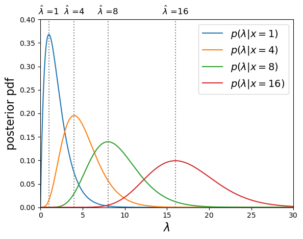
Poisson posterior distribution MLEs are equal to the observed rate.

The mean of the posterior distribution \(\langle \lambda \rangle\) is larger than the MLE (which is equivalent to the mode of the distribution, because the distribution is positively skewed (i.e. skewed to the right). However, over many repeated experiments with the same rate parameter \(\lambda_{\mathrm{true}}\), \(E[\langle \lambda \rangle]=\lambda_{\mathrm{true}}+1\), while \(E[\hat{\lambda}]=\lambda_{\mathrm{true}}\). I.e. the mean of the posterior distribution is a biased estimator in this case, while the MLE is not.

Errors on MLEs

It’s important to remember that the MLE \(\hat{\theta}\) is only an estimator for the true parameter value \(\theta_{\mathrm{true}}\), which is contained somewhere in the posterior probability distribution for \(\theta\), with probability of it occuring in a certain range, given by integrating the distribution over that range, as is the case for the pdf of a random variable. Previously, we looked at the approach of using the posterior distribution to define confidence intervals. Now we will examine a simpler approach to estimating the error on an MLE, which is exact for the case of a posterior which is a normal distribution.

Consider a log-likelihood \(L(\theta)\) with maximum at the MLE, at \(L(\hat{\theta})\). We can examine the shape of the probability distribution of \(\theta\) around \(\hat{\theta}\) by expanding \(L(\theta)\) about the maximum:

where the 1st order term is zero because \(\frac{\mathrm{d}L}{\mathrm{d}\theta}\bigg\rvert_{\hat{\theta}} = 0\) at \(\theta=\hat{\theta}\), by definition.

For smooth log-likelihoods, where we can neglect the higher order terms, the distribution around the MLE can be approximated by a parabola with width dependent on the 2nd derivative of the log-likelihood. To see what this means, lets transform back to the probability, \(p(\theta)=\exp\left(L(\theta)\right)\):

The equation on the right hand side should be familiar to us: it is the normal distribution!

i.e. for smooth log-likelihood functions, the posterior probability distribution of the parameter \(\theta\) can be approximated with a normal distribution about the MLE \(\hat{\theta}\), i.e. with mean \(\mu=\hat{\theta}\) and variance \(\sigma^{2}=-\left(\frac{\mathrm{d}^{2}L}{\mathrm{d}\theta^{2}}\bigg\rvert_{\hat{\theta}}\right)^{-1}\). Thus, assuming this Gaussian or normal approximation , we can estimate a 1-\(\sigma\) uncertainty or error on \(\theta\) which corresponds to a range about the MLE value where the true value should be \(\simeq\)68.2% of the time:

How accurate this estimate for \(\sigma\) is will depend on how closely the posterior distribution approximates a normal distribution, at least in the region of parameter values that contains most of the probability. The estimate will become exact in the case where the posterior is normally distributed.

Test yourself: errors on Binomial and Poisson MLEs

Use the normal approximation to estimate the standard deviation on the MLE for binomial and Poisson distributed likelihood functions, in terms of the observed data (\(x\) successes in \(n\) trials, or \(x\) counts).

Solution

For the binomial distribution we have already shown that: \(\frac{\mathrm{d}L}{\mathrm{d}\theta} = \frac{x}{\theta} - \frac{n-x}{(1-\theta)} \quad \rightarrow \quad \frac{\mathrm{d}^{2}L}{\mathrm{d}\theta^{2}}\bigg\rvert_{\hat{\theta}} = -\frac{x}{\hat{\theta}^{2}} - \frac{n-x}{(1-\hat{\theta})^{2}} = -\frac{n}{\hat{\theta}(1-\hat{\theta})}\)

So we obtain: \(\sigma = \sqrt{\frac{\hat{\theta}(1-\hat{\theta})}{n}}\) and since \(\hat{\theta}=x/n\) our final result is: \(\sigma = \sqrt{\frac{x(1-x/n)}{n^2}}\)

For the Poisson distributed likelihood we already showed in a previous challenge that \(\frac{\mathrm{d}^{2}L}{\mathrm{d}\lambda^{2}}\bigg\rvert_{\hat{\lambda}} = - \frac{x}{\hat{\lambda}^{2}}\) and \(\hat{\lambda}=x\)

So, \(\sigma = \sqrt{x}\).

Using optimisers to obtain MLEs

For the distributions discussed so far, the MLEs could be obtained analytically from the derivatives of the likelihood function. However, in most practical examples, the data are complex (i.e. multiple measurements) and the model distribution may include multiple parameters, making an analytical solution impossible. In some cases, like those we have examined so far, it is possible to calculate the posterior distribution numerically. However, that can be very challenging when considering complex data and/or models with many parameters, leading to a multi-dimensional parameter hypersurface which cannot be efficiently mapped using any kind of computation over a dense grid of parameter values. Furthermore, we may only want the MLEs and perhaps their errors, rather than the entire posterior pdf. In these cases, where we do not need or wish to calculate the complete posterior distribution, we can obtain the MLEs numerically, via a numerical approach called optimisation.

Optimisation methods use algorithmic approaches to obtain either the minimum or maximum of a function of one or more adjustable parameters. These approaches are implemented in software using optimisers. We do not need the normalised posterior pdf in order to obtain an MLE, since only the pdf shape matters to find the peak. So the function to be optimised is often the likelihood function (for the uniform prior case) or product of likelihood and prior, or commonly some variant of those, such as the log-likelihood or, as we will see later weighted least squares, colloquially known as chi-squared fitting.

Optimisation methods and the scipy.optimize module.

There are a variety of optimisation methods which are available in Python’s scipy.optimize module. Many of these approaches are discussed in some detail in Chapter 10 of the book ‘Numerical Recipes’, available online here. Here we will give a brief summary of some of the main methods and their pros and cons for maximum likelihood estimation. An important aspect of most numerical optimisation methods, including the ones in scipy, is that they are minimisers, i.e. they operate to minimise the given function rather than maximise it. This works equally well for maximising the likelihood, since we can simply multiply the function by -1 and minimise it to achieve our maximisation result.

• Scalar minimisation: the function scipy.optimize.minimize_scalar has several methods for minimising functions of only one variable. The methods can be specified as arguments, e.g. method='brent' uses Brent’s method of parabolic interpolation: find a parabola between three points on the function, find the position of its minimum and use the minimum to replace the highest point on the original parabola before evaluating again, repeating until the minimum is found to the required tolerance. The method is fast and robust but can only be used for functions of 1 parameter and as no gradients are used, it does not return the useful 2nd derivative of the function.
• Downhill simplex (Nelder-Mead): scipy.optimize.minimize offers the method nelder-mead for rapid and robust minimisation of multi-parameter functions using the ‘downhill simplex’ approach. The approach assumes a simplex, an object of \(n+1\) points or vertices in the \(n\)-dimensional parameter space. The function to be minimised is evaluated at all the vertices. Then, depending on where the lowest-valued vertex is and how steep the surrounding ‘landscape’ mapped by the other vertices is, a set of rules are applied to move one or more points of the simplex to a new location. E.g. via reflection, expansion or contraction of the simplex or some combination of these. In this way the simplex ‘explores’ the \(n\)-dimensional landscape of function values to find the minimum. Also known as the ‘amoeba’ method because the simplex ‘oozes’ through the landscape like an amoeba!
• Gradient methods: a large set of methods calculate the gradients or even second derivatives of the function (hyper)surface in order to quickly converge on the minimum. A commonly used example is the Broyden-Fletcher-Goldfarb-Shanno (BFGS) method (method=BFGS in scipy.optimize.minimize or the legacy function scipy.optimize.fmin_bfgs). A more specialised function using a variant of this approach which is optimised for fitting functions to data with normally distributed errors (‘weighted non-linear least squares’) is scipy.optimize.curve_fit. The advantage of these functions is that they usually return either a matrix of second derivatives (the ‘Hessian’) or its inverse, which is the covariance matrix of the fitted parameters. These can be used to obtain estimates of the errors on the MLEs, following the normal approximation approach described in this episode.

An important caveat to bear in mind with all optimisation methods is that for finding minima in complicated hypersurfaces, there is always a risk that the optimiser returns only a local minimum, end hence incorrect MLEs, instead of those at the true minimum for the function. Most optimisers have built-in methods to try and mitigate this problem, e.g. allowing sudden switches to completely different parts of the surface to check that no deeper minimum can be found there. It may be that a hypersurface is too complicated for any of the optimisers available. In this case, you should consider looking at Markov Chain Monte Carlo methods to fit your data.

In the remainder of this course we will use the Python package lmfit which combines the use of scipy’s optimisation methods with some powerful functionality to control model fits and determine errors and confidence contours.

General maximum likelihood estimation: model fitting

So far we have only considered maximum likelihood estimation applied to simple univariate models and data. It’s much more common in the physical sciences that our data is (at least) bivariate i.e. \((x,y)\) and that we want to fit the data with multi-parameter models. We’ll look at this problem in this episode.

First consider our hypothesis, consisting of a physical model relating a response variable \(y\) to some explanatory variable \(x\). There are \(n\) pairs of measurements, with a value \(y_{i}\) corresponding to each \(x_{i}\) value, \(x_{i}=x_{1},x_{2},...,x_{n}\). We can write both sets of values as vectors, denoted by bold fonts: \(\mathbf{x}\), \(\mathbf{y}\).

Our model is not completely specified, some parameters are unknown and must be obtained from fitting the model to the data. The \(M\) model parameters can also be described by a vector \(\pmb{\theta}=[\theta_{1},\theta_{2},...,\theta_{M}]\).

Now we bring in our statistical model. Assuming that the data are unbiased, the model gives the expectation value of \(y\) for a given \(x\) value and model parameters, i.e. it gives \(E[y]=f(x,\pmb{\theta})\). The data are assumed to be independent and drawn from a probability distribution with expectation value given by the model, and which can be used to calculate the probability of obtaining a data \(y\) value given the corresponding \(x\) value and model parameters: \(p(y_{i}\vert x_{i}, \pmb{\theta})\).

Since the data are independent, their probabilities are multiplied together to obtain a total probability for a given set of data, under the assumed hypothesis. The likelihood function is:

So that the log-likelihood is:

and to obtain the MLEs for the model parameters, we should maximise the value of his log-likelihood function. This procedure of finding the MLEs of model parameters via maximising the likelihood is often known more colloquially as model fitting (i.e. you ‘fit’ the model to the data).

MLEs and errors from multi-parameter model fitting

When using maximum likelihood to fit a model with multiple (\(M\)) parameters \(\pmb{\theta}\), we obtain a vector of 1st order partial derivatives, known as scores:

i.e. \(U(\pmb{\theta})=\nabla L\). In vector calculus we call this vector of 1st order partial derivatives the Jacobian. The MLEs correspond to the vector of parameter values where the scores for each parameter are zero, i.e. \(U(\hat{\pmb{\theta}})= (0,...,0) = \mathbf{0}\).

We saw in the previous episode that the variances of these parameters can be derived from the 2nd order partial derivatives of the log-likelihood. Now let’s look at the case for a function of two parameters, \(\theta\) and \(\phi\). The MLEs are found where:

where we use \(L=L(\phi,\theta)\) for convenience. Note that the maximum corresponds to the same location for both MLEs, so is evaluated at \(\hat{\theta}\) and \(\hat{\phi}\), regardless of which parameter is used for the derivative. Now we expand the log-likelihood function to 2nd order about the maximum (so the first order term vanishes):

The ‘error’ term in the square brackets is the equivalent for 2-parameters to the 2nd order term for one parameter which we saw in the previous episode. This term may be re-written using a matrix equation:

where \(A = \frac{\partial^{2}L}{\partial\theta^{2}}\bigg\rvert_{\hat{\theta},\hat{\phi}}\), \(B = \frac{\partial^{2}L}{\partial\phi^{2}}\bigg\rvert_{\hat{\theta},\hat{\phi}}\) and \(C=\frac{\partial^{2}L}{\partial\theta \partial\phi}\bigg\rvert_{\hat{\theta},\hat{\phi}}\). Since \(L(\hat{\theta},\hat{\phi})\) is a maximum, we require that \(A<0\), \(B<0\) and \(AB>C^{2}\).

This approach can also be applied to models with \(M\) parameters, in which case the resulting matrix of 2nd order partial derivatives is \(M\times M\). In vector calculus terms, this matrix of 2nd order partial derivatives is known as the Hessian. As could be guessed by analogy with the result for a single parameter in the previous episode, we can directly obtain estimates of the variance of the MLEs by taking the negative inverse matrix of the Hessian of our log-likelihood evaluated at the MLEs. In fact, this procedure gives us the covariance matrix for the MLEs. For our 2-parameter case this is:

The diagonal terms of the covariance matrix give the marginalised variances of the parameters, so that in the 2-parameter case, the 1-\(\sigma\) errors on the parameters (assuming the normal approximation, i.e. normally distributed likelihood about the maximum) are given by:

The off-diagonal term is the covariance of the errors between the two parameters. If it is non-zero, then the errors are correlated, e.g. a deviation of the MLE from the true value of one parameter causes a correlated deviation of the MLE of the other parameter from its true value. If the covariance is zero (or negligible compared to the product of the parameter errors), the errors on each parameter reduce to the same form as the single-parameter errors described above, i.e.:

Weighted least squares: ‘chi-squared fitting’

Let’s consider the case where the data values \(y_{i}\) are drawn from a normal distribution about the expectation value given by the model, i.e. we can define the mean and variance of the distribution for a particular measurement as:

and the standard deviation \(\sigma_{i}\) is given by the error on the data value. Note that this situation is not the same as in the normal approximation discussed above, since here it is the data which are normally distributed, not the likelihood function.

The likelihood function for the data points is:

and the log-likelihood is:

Note that the first term on the RHS is a constant defined only by the errors on the data, while the second term is the sum of squared residuals of the data relative to the model, normalised by the squared error of the data. This is something we can easily calculate without reference to probability distributions! We therefore define a new statistic \(X^{2}(\pmb{\theta})\):

This statistic is often called the chi-squared (\(\chi^{2}\)) statistic, and the method of maximum likelihood fitting which uses it is formally called weighted least squares but informally known as ‘chi-squared fitting’ or ‘chi-squared minimisation’. The name comes from the fact that, where the model is a correct description of the data, the observed \(X^{2}\) is drawn from a chi-squared distribution. Minimising \(X^{2}\) is equivalent to maximising \(L(\pmb{\theta})\) or \(l(\pmb{\theta})\). In the case where the error is identical for all data points, minimising \(X^{2}\) is equivalent to minimising the sum of squared residuals in linear regression.

The chi-squared distribution

Consider a set of independent variates drawn from a standard normal distribution, \(Z\sim N(0,1)\): \(Z_{1}, Z_{2},...,Z_{n}\).

We can form a new variate by squaring and summing these variates: \(X=\sum\limits_{i=1}^{n} Z_{i}^{2}\)

The resulting variate \(X\) is drawn from a \(\chi^{2}\) (chi-squared) distribution:

\[p(x\vert \nu) = \frac{(1/2)^{\nu/2}}{\Gamma(\nu/2)}x^{\frac{\nu}{2}-1}e^{-x/2}\]

where \(\nu\) is the distribution shape parameter known as the degrees of freedom, as it corresponds to the number of standard normal variates which are squared and summed to produce the distribution. \(\Gamma\) is the Gamma function. Note that for integers \(\Gamma(n)=(n-1)!\) and for half integers \(\Gamma(n+\frac{1}{2})=\frac{(2n)!}{4^{n}n!} \sqrt{\pi}\). Therefore, for \(\nu=1\), \(p(x)=\frac{1}{\sqrt{2\pi}}x^{-1/2}e^{-x/2}\). For \(\nu=2\) the distribution is a simple exponential: \(p(x)=\frac{1}{2} e^{-x/2}\). Since the chi-squared distribution is produced by sums of \(\nu\) random variates, the central limit theorem applies and for large \(\nu\), the distribution approaches a normal distribution.

A variate \(X\) which is drawn from chi-squared distribution, is denoted \(X\sim \chi^{2}_{\nu}\) where the subscript \(\nu\) is given as an integer denoting the degrees of freedom. Variates distributed as \(\chi^{2}_{\nu}\) have expectation \(E[X]=\nu\) and variance \(V[X]=2\nu\).

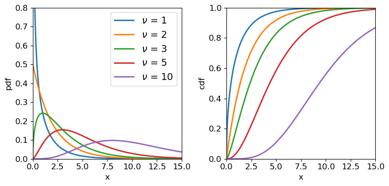
Chi-squared distributions for different degrees of freedom.

Weighted least squares estimation in Python with the lmfit package

We already saw how to use Scipy’s curve_fit function to carry out a linear regression fit with error bars on \(y\) values not included. The curve_fit routine uses non-linear least-squares to fit a function to data (i.e. it is not restricted to linear least-square fitting) and if the error bars are provided it will carry out a weighted-least-squares fit, which is what we need to obtain a goodness-of-fit (see below). As well as returning the MLEs, curve_fit also returns the covariance matrix evaluated at the minimum chi-squared, which allows errors on the MLEs to be estimated. However, while curve_fit can be used on its own to fit models to data and obtain MLEs and their errors, we will instead carry out weighted least squares estimation using the Python lmfit package, which enables a range of optimisiation methods to be used and provides some powerful functionality for fitting models to data and determining errors. We will use lmfit throughout the reminder of this course. It’s documentation can be found here, but it can be difficult to follow without some prior knowledge of the statistical methods being used. Therefore we advise you first to follow the tutorials given in this and the following episodes, before following the lmfit online documentation for a more detailed understanding of the package and its capabilities.

Model fitting with lmfit, in a nutshell

Lmfit can be used to fit models to data by minimising the output (or sum of squares of the output) of a so-called objective function, which the user provides for the situation being considered. For weighted least squares, the objective function calculates and returns a vector of weighted residuals \((y_{i} - y_{\rm model}(x_{i}))/err(y_{i})\), while for general maximum likelihood estimation, the objective function should return a scalar quantity, such as the negative log-likelihood. The inputs to the objective function are the model itself (e.g. the name of a separate model function), the data (\(x\) and \(y\) values and \(y\) errors), a special Parameters object which contains and controls the model parameters to be estimated (or assumed) and any other arguments to be used by the objective function. Lmfit is a highly developed package with considerably more (and more complex) functionality and classes than we will outline here. However, for simplicity and the purpose of this course, we present below some streamlined information about the classes which we will use for fitting models to data in this and following episodes.

• The Parameters object is a crucial feature of lmfit which enables quite complex constraints to be applied to the model parameters, e.g. freezing some and freeing others, or setting bounds which limit the range of parameter values to be considered by the fit, or even defining parameters using some expression of one or more of the other model parameters. A Parameters object is a dictionary of a number of separate Parameter objects (one per parameter) with keywords corresponding to the properties of the parameter, such as the value (which can be used to set the starting value or return the current value), vary (set True or False if the parameter is allowed to vary in the fit or is frozen at a fixed value), and min or max to set bounds. The Parameters object name must be the first argument given to the objective function that is minimised.
• The Minimizer object is used to set up the minimisation approach to be used. This includes specifying the objective function to be used, the associated Parameters object and any other arguments and keywords used by the objective function. Lmfit can use a wide variety of minimisation approaches from Scipy’s optimize module as well as other modules (e.g. emcee for Markov Chain Monte Carlo - MCMC - fitting) and the approach to be used (and any relevant settings) are also specified when assigning a Minimizer object. The minimisation (i.e. the fit) is itself done by applying the minimize() method to the Minimizer object.
• The results of the fit (and more besides) are given by the MinimizerResult object, which is produced as the output of the minimize() method and includes the best-fitting parameter values (the MLEs), the best-fitting value(s) of the objective function and (if determined) the parameter covariance matrix, chi-squared and degrees of freedom and possibly other test statistics. Note that the MinimizerResult and Minimizer objects can also be used in other functions, e.g. to produce confidence contour plots or other useful outputs.

Fitting the energy-dependence of the pion-proton scattering cross-section

Resonances in the pion-proton (\(\pi^{+}\)-\(p\) interaction provided important evidence for the existence of quarks. One such interaction was probed in an experiment described by Pedroni et al. (1978):

which describes the scattering producing a short-lived resonance particle (\(\Delta^{++}(1232)\)) which decays back into the original particles. Using a beam of pions with adjustable energy, the experimenters were able to measure the scattering cross-section \(\sigma\) (in mb) as a function of beam energy in MeV. These data, along with the error on the cross-section, are provided in the file pedroni_data.txt, here.

First we will load the data. Here we will use numpy.genfromtxt which will load the data to a structured array with columns identifiable by their names. We will only use the 1st three columns (beam energy, cross-section and error on cross-section). We also select energies \(<=313\) MeV, as recommended by Pedroni et al. and since the data are not already ordered by energy, we sort the data array by energy (having a numerically ordered set of \(x\)-axis values is useful for plotting purposes, but not required by the method).

pion = np.genfromtxt('pedroni.txt', dtype='float', usecols=(0,1,2), names=True)
# Now sort by energy and ignore energies > 313 MeV 
pion_clean = np.sort(pion[pion['energy'] <= 313], axis=0)
print(pion_clean.dtype.names) # Check field names for columns of structured array

('energy', 'xsect', 'error')

The resonant energy of the interaction, \(E_{0}\) (in MeV), is a key physical parameter which can be used to constrain physical models. For these data it can be obtained by modelling the cross-section using the non-relativistic Breit-Wigner formula:

where \(\sigma(E)\) is the energy-dependent cross-section, \(N\) is a normalisation factor and \(\Gamma\) is the resonant interaction ‘width’ (also in MeV), which is inversely related to the lifetime of the \(\Delta^{++}\) resonance particle. This lifetime is a function of energy, such that:

where \(\Gamma_{0}\) is the width at 130 MeV. Thus we finally have a model for \(\sigma(E)\) with \(N\), \(E_{0}\) and \(\Gamma_{0}\) as its unknown parameters.

To use this model to fit the data with lmfit, we’ll first import lmfit and the subpackages Minimizer and report_fit. Then we’ll define a Parameter object, which we can use as input to the model function and objective function.

import lmfit
from lmfit import Minimizer, Parameters, report_fit

params = Parameters()  # Assigns a variable name to an empty Parameters object
params.add_many(('gam0',30),('E0',130),('N',150))  # Adds multiple parameters, specifying the name and starting value

The initial parameter values (here \(\Gamma_{0}=30\) MeV, \(E_{0}=130\) MeV and \(N=150\) mb) need to be chosen so that they are not so far away from the best-fitting parameters that the fit will get stuck, e.g. in a local-minimum, or diverge in the wrong direction away from the best-fitting parameters. You may have a physical motivation for a good choice of starting parameters, but it is also okay to plot the model on the same plot as the data and tweak the parameters so the model curve is at least not too far from most of the data. For now we only specified the values associated with the name and value keywords. We will use other Parameter keywords in the next episodes. We can output a dictionary of the name and value pairs, and also a tabulated version of all the parameter properties, using the valuesdict and pretty_print methods respectively:

print(params.valuesdict())
params.pretty_print()

{'gam0': 30, 'E0': 130, 'N': 150}
Name     Value      Min      Max   Stderr     Vary     Expr Brute_Step
E0         130     -inf      inf     None     True     None     None
N          150     -inf      inf     None     True     None     None
gam0        30     -inf      inf     None     True     None     None

We will discuss some of the other parameter properties given in the tabulated output (and currently set to the defaults) later on.

Now that we have defined our Parameters object we can use it as input for a model function which returns a vector of model \(y\) values for a given vector of \(x\) values, in this case the \(x\) values are energies e_val and the function is the version of the Breit-Wigner formula given above.

def breitwigner(e_val,params):
    '''Function for non-relativistic Breit-Wigner formula, returns pi-p interaction cross-section
    for input energy and parameters resonant width, resonant energy and normalisation.'''
    v = params.valuesdict()
    gam=v['gam0']*np.sqrt(e_val/130.)
    return v['N']*(gam**2/4)/((e_val-v['E0'])**2+gam**2/4)

Note that the variables are given by using the valuesdict method together with the parameter names given when assigning the Parameters object.

Next, we need to set up our lmfit objective function, which we will do specifically for weighted least squares fitting, so the output should be the array of weighted residuals. We want our function to be quite generic and enable simultaneous fitting of any given model to multiple data sets (which we will learn about in two Episodes time). The main requirement from lmfit, besides the output being the array of weighted residuals, is that the first argument should be the Parameters object used by the fit. Beyond that, there are few restrictions except the usual rule that function positional arguments are followed by keyword arguments (i.e. in formal Python terms, the objective function fcn is defined as fcn(params, *args, **kws)). Therefore we choose to enter the data as lists of arrays: xdata, ydata and yerrs, and we also give the model function name as an argument model (so that the objective function can be calculated with any model chosen by the user). Note that for minimization the residuals for different data sets will be concatenated into a single array, but for plotting purposes we would also like to have the option to use the function to return a list-of-arrays format of the calculated model values for our input data arrays. So we include that possibility of changing the output by using a Boolean keyword argument output_resid, which is set to True as a default to return the objective function output for minimisation.

def lmf_lsq_resid(params,xdata,ydata,yerrs,model,output_resid=True):
    '''lmfit objective function to calculate and return residual array or model y-values.
        Inputs: params - name of lmfit Parameters object set up for the fit.
                xdata, ydata, yerrs - lists of 1-D arrays of x and y data and y-errors to be fitted.
                    E.g. for 2 data sets to be fitted simultaneously:
                        xdata = [x1,x2], ydata = [y1,y2], yerrs = [err1,err2], where x1, y1, err1
                        and x2, y2, err2 are the 'data', sets of 1-d arrays of length n1, n2 respectively, 
                        where n1 does not need to equal n2.
                    Note that a single data set should also be given via a list, i.e. xdata = [x1],...
                model - the name of the model function to be used (must take params as its input params and
                        return the model y-value array for a given x-value array).
                output_resid - Boolean set to True if the lmfit objective function (residuals) is
                        required output, otherwise a list of model y-value arrays (corresponding to the 
                        input x-data list) is returned.
        Output: if output_resid==True, returns a residual array of (y_i-y_model(x_i))/yerr_i which is
            concatenated into a single array for all input data errors (i.e. length is n1+n2 in 
            the example above). If output_resid==False, returns a list of y-model arrays (one per input x-array)'''
    if output_resid == True:
        for i, xvals in enumerate(xdata):  # loop through each input dataset and record residual array
            if i == 0:
                resid = (ydata[i]-model(xdata[i],params))/yerrs[i]
            else:
                resid = np.append(resid,(ydata[i]-model(xdata[i],params))/yerrs[i])
        return resid
    else:
        ymodel = []
        for i, xvals in enumerate(xdata): # record list of model y-value arrays, one per input dataset
            ymodel.append(model(xdata[i],params))
        return ymodel

Of course, you can always set up the objective function in a different way if you prefer it, or to better suit what you want to do. The main thing is to start the input arguments with the Parameters object and return the correct output for minimization (a single residual array in this case).

Now we can fit our data! We do this by first assigning some of our input variables (note that here we assign the data arrays as items in corresponding lists of \(x\), \(y\) data and errors, as required by our pre-defined objective function). Then we create a Minimizer object, giving as arguments our objective function name, parameters object name and keyword argument fcn_args (which requires a tuple of the other arguments that go into our objective function, after the parameter object name). We also use a keyword argument nan_policy to omit NaN values in the data from the calculation (although that is not required here, it may be useful in future).

Once the fit has been done (by applying the minimize method with the optimisation approach set to leastsq), we use the output with the lmfit function report_fit, to output (among other things) the minimum weighted-least squares value (so-called ‘chi-squared’) and the best-fitting parameters (i.e. the parameter MLEs) and their estimated 1-\(\sigma\) (\(68\%\) confidence interval) errors, which are determined using the numerical estimate of 2nd-order partial derivatives of the weighted-least squares function (\(\equiv -\)ve log-likelihood) at the minimum (i.e. the approach described in this episode). The errors should be accurate if the likelihood for the parameters is close to a multivariate normal distribution. The correlations are calculated from the covariance matrix of the parameters, i.e. they give an indication of how well-correlated are the errors in the two parameters.

model = breitwigner
output_resid = True
xdata = [pion_clean['energy']]
ydata = [pion_clean['xsect']]
yerrs = [pion_clean['error']]
set_function = Minimizer(lmf_lsq_resid, params, fcn_args=(xdata, ydata, yerrs, model, output_resid), nan_policy='omit')
result = set_function.minimize(method = 'leastsq')
report_fit(result)

[[Fit Statistics]]
    # fitting method   = leastsq
    # function evals   = 34
    # data points      = 36
    # variables        = 3
    chi-square         = 38.0129567
    reduced chi-square = 1.15190778
    Akaike info crit   = 7.95869265
    Bayesian info crit = 12.7092495
[[Variables]]
    gam0:  110.227040 +/- 0.37736748 (0.34%) (init = 30)
    E0:    175.820915 +/- 0.18032507 (0.10%) (init = 130)
    N:     205.022251 +/- 0.52530542 (0.26%) (init = 150)
[[Correlations]] (unreported correlations are < 0.100)
    C(gam0, N)  = -0.690
    C(gam0, E0) = -0.344
    C(E0, N)    = -0.118

We can also plot our model and the \(data-model\) residuals to show the quality of the fit and assess whether there is any systematic mismatch between the model and the data:

# For plotting a smooth model curve we need to define a grid of energy values:
model_ens = np.linspace(50.0,350.0,1000)

# To calculate the best-fitting model values, use the parameters of the best fit output
# from the fit, result.params and set output_resid=false to output a list of model y-values:
model_vals = lmf_lsq_resid(result.params,[model_ens],ydata,yerrs,model,output_resid=False)

fig, (ax1, ax2) = plt.subplots(2,1, figsize=(8,6),sharex=True,gridspec_kw={'height_ratios':[2,1]})
fig.subplots_adjust(hspace=0)
# Plot data as points with y-errors
ax1.errorbar(pion_clean['energy'], pion_clean['xsect'], yerr=pion_clean['error'], marker="o", linestyle="")

# Plot the model as a continuous curve. The model values produced by our earlier function are an array stored 
# as an item in a list, so we need to use index 0 to specifically output the y model values array.
ax1.plot(model_ens, model_vals[0], lw=2)
ax1.set_ylabel("Cross-section (mb)", fontsize=16)
ax1.tick_params(labelsize=14)

# Plot the data-model residuals as points with errors. Here we calculate the residuals directly for each
# data point, again using the index 0 to access the array contained in the output list, which we can append at 
# the end of the function call:
ax2.errorbar(pion_clean['energy'],
             pion_clean['xsect']-lmf_lsq_resid(result.params,xdata,ydata,yerrs,model,output_resid=False)[0],
             yerr=pion_clean['error'],marker="o", linestyle="")

ax2.set_xlabel("Energy (MeV)",fontsize=16)
ax2.set_ylabel("Residuals (mb)", fontsize=16)
ax2.axhline(0.0, color='r', linestyle='dotted', lw=2) ## when showing residuals it is useful to also show the 0 line
ax2.tick_params(labelsize=14)
plt.show()

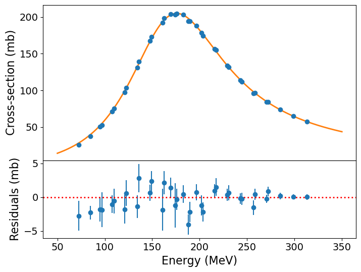
The model curve is clearly a good fit to the data, although the residuals show systematic deviations (up to a few times the error bar) for the cross-sections measured at lower beam energies. It is worth bearing in mind however that our treatment is fairly simplistic, using the non-relativistic version of the formula and ignoring instrumental background. So perhaps it isn’t surprising that we see some deviations. It remains useful to ask: how good is our fit anyway?

Goodness of fit

An important aspect of weighted least squares fitting is that a significance test, the chi-squared test can be applied to check whether the minimum \(X^{2}\) statistic obtained from the fit is consistent with the model being a good fit to the data. In this context, the test is often called a goodness of fit test and the \(p\)-value which results is called the goodness of fit. The goodness of fit test checks the hypothesis that the model can explain the data. If it can, the data should be normally distributed around the model and the sum of squared, weighted data\(-\)model residuals should follow a \(\chi^{2}\) distribution with \(\nu\) degrees of freedom. Here \(\nu=n-m\), where \(n\) is the number of data points and \(m\) is the number of free parameters in the model (i.e. the parameters left free to vary so that MLEs were determined).

It’s important to remember that the chi-squared statistic can only be positive-valued, and the chi-squared test is single-tailed, i.e. we are only looking for deviations with large chi-squared compared to what we expect, since that corresponds to large residuals, i.e. a bad fit. Small chi-squared statistics can arise by chance, but if it is so small that it is unlikely to happen by chance (i.e. the corresponding cdf value is very small), it suggests that the error bars used to weight the squared residuals are too large, i.e. the errors on the data are overestimated. Alternatively a small chi-squared compared to the degrees of freedom could indicate that the model is being ‘over-fitted’, e.g. it is more complex than is required by the data, so that the model is effectively fitting the noise in the data rather than real features.

Sometimes (as in the lmfit output shown above), you will see the ‘reduced chi-squared’ discussed. This is the ratio \(X^2/\nu\), written as \(\chi^{2}/\nu\) and also (confusingly) as \(\chi^{2}_{\nu}\). Since the expectation of the chi-squared distribution is \(E[X]=\nu\), a rule of thumb is that \(\chi^{2}/\nu \simeq 1\) corresponds to a good fit, while \(\chi^{2}/\nu\) greater than 1 are bad fits and values significantly smaller than 1 correspond to over-fitting or overestimated errors on data. It’s important to always bear in mind however that the width of the \(\chi^{2}\) distribution scales as \(\sim 1/\sqrt{\nu}\), so even small deviations from \(\chi^{2}/\nu = 1\) can be significant for larger numbers of data-points being fitted, while large \(\chi^{2}/\nu\) may arise by chance for small numbers of data-points. For a formal estimate of goodness of fit, you should determine a \(p\)-value calculated from the \(\chi^{2}\) distribution corresponding to \(\nu\).

Let’s calculate the goodness of fit of the non-relativistic Breit-Wigner formula to our data. To do so we need the best-fitting chi-squared and the number of degrees of freedom. We can access these from our fit result and use them to calculate the goodness of fit:

print("Minimum Chi-squared = "+str(result.chisqr)+" for "+str(result.nfree)+" d.o.f.")
print("The goodness of fit is: ",sps.chi2.sf(result.chisqr,df=result.nfree))

Minimum Chi-squared = 38.01295670804502 for 33 d.o.f.
The goodness of fit is:  0.25158686748918946

Our \(p\)-value (goodness of fit) is 0.25, indicating that the data are consistent with being normally distributed around the model, according to the size of the data errors. I.e., the fit is good. This does not mean it can’t be improved however, e.g. by a more complex model with additional free parameters. We will discuss this issue in a couple of episodes’ time.

Programming challenge: fitting binary pulsar timing data

The file pulsar-timing.txt contains data on the timing of the binary pulsar PSR~1913+16. The data are from Taylor & Weisberg (1982; Astrophysical Journal, v235, pp.908-920). They show the “orbit phase residuals” from precise timing of the orbit of the system. The first column shows the observation, the second the date (in years) the third column shows the phase residual in years and the fourth column shows the error on the phase residual (also years). You can assume that the errors are normally distributed.

If the orbit was (a) constant (at 7.76 hours) the residuals should be constant with time. If the orbit was (b) constant but its period was incorrectly determined the residuals should grow linearly with time. If the period of the system is constantly changing (c) there should be a parabolic change in the residual with time. A constantly increasing period (a quadratically decreasing phase residual) is what we would expect if gravitational waves are radiating energy from the system.

Use weighted least squares fitting with lmfit to fit the following models to the data and obtain MLEs of the model parameters and their 1\(-\sigma\) errors. By plotting the data and best-fitting models and data-model residuals, and also determining a goodness-of-fit for each model, decide which model or models give a reasonable match to the data:

• a. A constant: \(y=\alpha\)
• b. A linear function: \(y=\alpha+\beta x\)
• c. A quadratic function: \(y=\alpha+\beta x+\gamma x^{2}\)

Key Points

• Given a set of data and a model with free parameters, the best unbiased estimators of the model parameters correspond to the maximum likelihood and are called Maximum Likelihood Estimators (MLEs).

• In the case of normally-distributed data, the log-likelihood is formally equivalent to the weighted least squares statistic (also known as the chi-squared statistic).

• MLEs can be obtained by maximising the (log-)likelihood or minimising the weighted least squares statistic (chi-squared minimisation).

• The Python package lmift can be used to fit data efficiently, and the leastsq minimisation method is optimised to carry out weighted least-squares fitting of models to data.

• The errors on MLEs can be estimated from the diagonal elements of the covariance matrix obtained from the fit, if the fitting method returns it. These errors are returned directly in the case of lmfit using