1. Introducing probability and discrete random variables

Overview

Teaching: 60 min
Exercises: 60 min

Questions

• How do we describe discrete random variables and what are their common probability distributions?

• How do I calculate the means, variances and other statistical quantities for numbers drawn from probability distributions?

Objectives

• Learn the definitions of events, sample spaces and independence.

• Learn how discrete random variables are defined and how the Bernoulli, binomial and Poisson distributions are derived from them.

• Learn how the expected means and variances of discrete random variables (and functions of them) can be calculated from their probability distributions.

• Plot, and carry out probability calculations with the binomial and Poisson distributions.

• Carry out simple simulations using random variables drawn from the binomial and Poisson distributions

In this episode we will be using numpy, as well as matplotlib’s plotting library. Scipy contains an extensive range of probability distributions in its ‘scipy.stats’ module, so we will also need to import it. Remember: scipy modules should be installed separately as required - they cannot be called if only scipy is imported.

import numpy as np
import matplotlib.pyplot as plt
import scipy.stats as sps

Probability, and frequentist vs. Bayesian approaches

Correct statistical inference requires an understanding of probability and how to work with it. We can do this using the language of mathematics and probability theory.

First let us consider what a probability is. There are two approaches to this, famously known as the frequentist and Bayesian approaches:

• A frequentist approach considers that the probability \(P\) of a random event occuring is equivalent to the frequency such an event would occur at, in an infinite number of repeating trials which have that event as one of the outcomes. \(P\) is expressed as the fractional number of occurrences, relative to the total number. For example, consider the flip of a coin (which is perfect so it cannot land on it’s edge, only on one of its two sides). If the coin is fair (unbiased to one side or the other), it will land on the ‘heads’ side (denoted by \(H\)) exactly half the time in an infinite number of trials, i.e. the probability \(P(H)=0.5\).
• A Bayesian approach considers the idea of an infinite number of trials to be somewhat abstract: instead the Bayesian considers the probability \(P\) to represent the belief that we have that the event will occur. In this case we can again state that \(P(H)=0.5\) if the coin is fair, since this is what we expect. However, the approach also explicitly allows the experimenter’s prior belief in a hypothesis (e.g. ‘The coin is fair?’) to factor in to the assessment of probability. This turns out to be crucial to assessing the probability that a given hypothesis is true.

Some years ago these approaches were seen as being in conflict, but the value of ‘Bayesianism’ in answering scientific questions, as well as in the rapidly expanding field of Machine Learning, means it is now seen as the best approach to statistical inference. We can still get useful insights and methods from frequentism however, so what we present here will focus on what is practically useful and may reflect a mix of both approaches. Although, at heart, we are all Bayesians now.

We will consder the details of Bayes’ theorem later on. But first, we must introduce probability theory, in terms of the concepts of sample space and events, conditional probability, probability calculus, and (in the next episodes) probability distributions.

Sample space

Imagine a sample space, \(\Omega\) which contains the set of all possible and mutially exclusive outcomes of some random process (also known as elements or elementary outcomes of the set). In statistical terminology, an event is a set containing one or more outcomes. The event occurs if the outcome of a draw (or sample) of that process is in that set. Events do not have to be mutually exclusive and may also share outcomes, so that events may also be considered as combinations or subsets of other events.

For example, we can denote the sample space of the results (Heads, Tails) of two successive coin flips as \(\Omega = \{HH, HT, TH, TT\}\). Each of the four outcomes of coin flips can be seen as a separate event, but we can also can also consider new events, such as, for example, the event where the first flip is heads \(\{HH, HT\}\), or the event where both flips are the same \(\{HH, TT\}\).

Trials and samples

In the language of statistics a trial is a single ‘experiment’ to produce a set of one or more measurements, or in purely statistical terms, a single realisation of a sampling process, e.g. the random draw of one or more outcomes from a sample space. The result of a trial is to produce a sample. It is important not to confuse the sample size, which is the number of outcomes in a sample (i.e. produced by a single trial) with the number of trials. An important aspect of a trial is that the outcome is independent of that of any of the other trials. This need not be the case for the measurements in a sample which may or may not be independent.

Some examples are:

• A roll of a pair of dice would be a single trial. The sample size is 2 and the sample would be the numbers on the dice. It is also possible to consider that a roll of a pair of dice is two separate trials for a sample of a single dice (since the outcome of each is presumably independent of the other roll).
• A single sample of fake data (e.g. from random numbers) generated by a computer would be a trial. By simulating many trials, the distribution of data expected from complex models could be generated.
• A full deal of a deck of cards (to all players) would be a single trial. The sample would be the hands that are dealt to all the players, and the sample size would be the number of players. Note that individual players’ hands cannot themselves be seen as trials as they are clearly not independent of one another (since dealing from a shuffled deck of cards is sampling without replacement).

Test yourself: dice roll sample space

Write out as a grid the sample space of the roll of two six-sided dice (one after the other), e.g. a roll of 1 followed by 3 is denoted by the element 13. You can neglect commas for clarity. For example, the top row and start of the next row will be:

\[11\:21\:31\:41\:51\:61\] \[12\:22\:...........\]

Now highlight the regions corresponding to:

• Event \(A\): the numbers on both dice add up to be \(>\)8.
• Event \(B\): both dice roll the same number (e.g. two ones, two twos etc.).

Finally use your grid to calculate the probabilities of \((A \mbox{ and } B)\) and \((A \mbox{ or } B)\), assuming that the dice are fair, so that all the outcomes of a roll of two dice are equally probable.

Solution

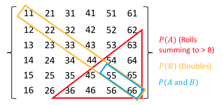
There are 36 possible outcomes, so assuming they are equally probable, a single outcome has a probability of 1/36 (\(\simeq\)0.028). We can see that the region corresponding to \(A \mbox{ and } B\) contains 2 outcomes, so \(P(A \mbox{ and } B)=2/36\). Region \(A\) contains 10 outcomes while region \(B\) contains 6. \(P(A \mbox{ or } B)\), which here corresponds to the number of unique outcomes, is given by: \(P(A)+P(B)-P(A \mbox{ and } B)=(10+6-2)/36=7/18\).

Rules of probability calculus 1

We can now write down two of rules of probability calculus and their extensions:

• The addition rule: \(P(A \mbox{ or } B) = P(A)+P(B)-P(A \mbox{ and } B)\)

\(A\) and \(B\) are independent if \(P(A \mbox{ and } B) = P(A)P(B)\).

We will consider the case where variables are not independent (we say they are conditional) later in the course.

Setting up a random event generator in Numpy

It’s often useful to generate your own random outcomes in a program, e.g. to simulate a random process or calculate a probability for some random event which is difficult or even impossible to calculate analytically. In this episode we will consider how to select a non-numerical outcome from a sample space. In the following episodes we will introduce examples of random number generation from different probability distributions.

Common to all these methods is the need for the program to generate random bits which are then used with a method to generate a given type of outcome. This is done in Numpy by setting up a generator object. A generic feature of computer random number generators is that they must be initialised using a random number seed which is an integer value that sets up the sequence of random numbers. Note that the numbers generated are not truly random: the sequence is the same if the same seed is used. However they are random with respect to one another. E.g.:

rng = np.random.default_rng(331)

will set up a generator with the seed=331. We can use this generator to produce, e.g. random integers to simulate five repeated rolls of a 6-sided dice:

print(rng.integers(1,7,5))
print(rng.integers(1,7,5))

where the first two arguments are the low and high (exclusive, i.e. 1 more than the maximum integer in the sample space) values of the range of contiguous integers to be sampled from, while the third argument is the size of the resulting array of random integers, i.e. how many outcomes to draw from the sample.

[1 3 5 3 6]
[2 3 2 2 6]

Note that repeating the command yields a different sample. This will be the case every time we repeat the integers function call, because the generator starts from a new point in the sequence. If we want to repeat the same ‘random’ sample we have to reset the generator to the same seed:

print(rng.integers(1,7,5))
rng = np.random.default_rng(331)
print(rng.integers(1,7,5))

[4 3 2 5 4]
[1 3 5 3 6]

For many uses of random number generators you may not care about being able to repeat the same sequence of numbers. In these cases you can set initialise the generator with the default seed using np.random.default_rng(), which obtains a seed from system information (usually contained in a continuously updated folder on your computer, specially for provide random information to any applications that need it). However, if you want to do a statistical test or simulate a random process that is exactly repeatable, you should consider specifying the seed. But do not initialise the same seed unless you want to repeat the same sequence!

Random sampling of items in a list or array

If you want to simulate random sampling of non-numerical or non-sequential elements in a sample space, a simple way to do this is to set up a list or array containing the elements and then apply the numpy method choice to the generator to select from the list. As a default, sampling probabilities are assumed to be \(1/n\) for a list with \(n\) items, but they may be set using the p argument to give an array of p-values for each element in the sample space. The replace argument sets whether the sampling should be done with or without replacement.

For example, to set up 10 repeated flips of a coin, for an unbiased and a biased coin:

rng = np.random.default_rng()  # Set up the generator with the default system seed
coin = ['h','t']
# Uses the defaults (uniform probability, replacement=True)
print("Unbiased coin: ",rng.choice(coin, size=10))
# Now specify probabilities to strongly weight towards heads:
prob = [0.9,0.1]
print("Biased coin: ",rng.choice(coin, size=10, p=prob))

Unbiased coin:  ['h' 'h' 't' 'h' 'h' 't' 'h' 't' 't' 'h']
Biased coin:  ['h' 'h' 't' 'h' 'h' 't' 'h' 'h' 'h' 'h']

Remember that your own results will differ from these because your random number generator seed will be different!

Discrete random variables

Often, we want to map a sample space \(\Omega\) (denoted with curly brackets) of possible outcomes on to a set of corresponding probabilities. The sample space may consist of non-numerical elements or numerical elements, but in all cases the elements of the sample space represent possible outcomes of a random ‘draw’ from a set of probabilities which can be used to form a discrete probability distribution.

For example, when flipping an ideal coin (which cannot land on its edge!) there are two outcomes, heads (\(H\)) or tails (\(T\)) so we have the sample space \(\Omega = \{H, T\}\). We can also represent the possible outcomes of 2 successive coin flips as the sample space \(\Omega = \{HH, HT, TH, TT\}\). A roll of a 6-sided dice would give \(\Omega = \{1, 2, 3, 4, 5, 6\}\). However, a Poisson process corresponds to the sample space \(\Omega = \mathbb{Z}^{0+}\), i.e. the set of all positive and integers and zero, even if the probability for most elements of that sample space is infinitesimal (it is still \(> 0\)).

In the case of a Poisson process or the roll of a dice, our sample space already consists of a set of contiguous (i.e. next to one another in sequence) numbers which correspond to discrete random variables. Where the sample space is categorical, such as heads or tails on a coin, or perhaps a set of discrete but non-integer values (e.g. a pre-defined set of measurements to be randomly drawn from), it is useful to map the elements of the sample space on to a set of integers which then become our discrete random variables. For example, when flipping a coin, we can define the possible values taken by the random variable, known as the variates \(X\), to be:

By defining the values taken by a random variable in this way, we can mathematically define a probability distribution for how likely it is for a given event or outcome to be obtained in a single trial (i.e. a draw - a random selection - from the sample space).

Probability distributions of discrete random variables

Random variables do not just take on any value - they are drawn from some probability distribution. In probability theory, a random measurement (or even a set of measurements) is an event which occurs (is ‘drawn’) with a fixed probability, assuming that the experiment is fixed and the underlying distribution being measured does not change over time (statistically we say that the random process is stationary).

We can write the probability that the variate \(X\) has a value \(x\) as \(p(x) = P(X=x)\), so for the example of flipping a coin, assuming the coin is fair, we have \(p(0) = p(1) = 0.5\). Our definition of mapping events on to random variables therefore allows us to map discrete but non-integer outcomes on to numerically ordered integers \(X\) for which we can construct a probability distribution. Using this approach we can define the cumulative distribution function or cdf for discrete random variables as:

where the subscript \(i\) corresponds to the numerical ordering of a given outcome, i.e. of an element in the sample space. For convenience we can also define the survival function, which is equal to \(P(X\gt x)\). I.e. the survival function is equal to \(1-F(x)\).

The function \(p(x)\) is specified for a given distribution and for the case of discrete random variables, is known as the probability mass function or pmf.

Properties of discrete random variates: mean and variance

Consider a set of repeated samples or draws of a random variable which are independent, which means that the outcome of one does not affect the probability of the outcome of another. A random variate is the quantity that is generated by sampling once from the probability distribution, while a random variable is the notional object able to assume different numerical values, i.e. the distinction is similar to the distinction in python between x=15 and the object to which the number is assigned x (the variable).

The expectation \(E(X)\) is equal to the arithmetic mean of the random variates as the number of sampled variates increases \(\rightarrow \infty\). For a discrete probability distribution it is given by the mean of the distribution function, i.e. the pmf, which is equal to the sum of the product of all possible values of the variable with the associated probabilities:

This quantity \(\mu\) is often just called the mean of the distribution, or the population mean to distinguish it from the sample mean of data, which we will come to later on.

More generally, we can obtain the expectation of some function of \(X\), \(f(X)\):

It follows that the expectation is a linear operator. So we can also consider the expectation of a scaled sum of variables \(X_{1}\) and \(X_{2}\) (which may themselves have different distributions):

and more generally for a scaled sum of variables \(Y=\sum\limits_{j} a_{j}X_{j}\):

i.e. the expectation for a scaled sum of variates is the scaled sum of their distribution means.

It is also useful to consider the variance, which is a measure of the squared ‘spread’ of the values of the variates around the mean, i.e. it is related to the weighted width of the probability distribution. It is a squared quantity because deviations from the mean may be positive (above the mean) or negative (below the mean). The (population) variance of discrete random variates \(X\) with (population) mean \(\mu\), is the expectation of the function that gives the squared difference from the mean:

It is possible to rearrange things:

In other words, the variance is the expectation of squares - square of expectations. Therefore, for a function of \(X\):

For a sum of independent, scaled random variables, the expected variance is equal to the sum of the individual variances multiplied by their squared scaling factors:

We will consider the case where the variables are correlated (and not independent) in a later Episode.

Test yourself: mean and variance of dice rolls

Starting with the probability distribution of the score (i.e. from 1 to 6) obtained from a roll of a single, fair, 6-sided dice, use equations given above to calculate the expected mean and variance of the total obtained from summing the scores from a roll of three 6-sided dice. You should not need to explicitly work out the probability distribution of the total from the roll of three dice!

Solution

We require \(E[Y]\) and \(V[Y]\), where \(Y=X+X+X\), with \(X\) the variate produced by a roll of one dice. The dice are fair so \(p(x)=P(X=x)=1/6\) for all \(X\) from 1 to 6. Therefore the expectation for one dice is \(E[X]=\frac{1}{6}\sum\limits_{i=1}^{6} i = 21/6 = 7/2\).

The variance is \(V[X]=E[X^{2}]-\left(E[X]\right)^{2} = \frac{1}{6}\sum\limits_{i=1}^{6} i^{2} - (7/2)^{2} = 91/6 - 49/4 = 35/12 \simeq 2.92\) .

The mean and variance for a roll of three six sided dice, since they are equally weighted is equal to the sums of mean and variance, i.e. \(E[Y]=21/2\) and \(V[Y]=35/4\).

Probability distributions: Bernoulli and Binomial

A Bernoulli trial is a draw from a sample with only two possibilities (e.g. the colour of sweets drawn, with replacement, from a bag of red and green sweets). The outcomes are mapped on to integer variates \(X=1\) or \(0\), assuming probability of one of the outcomes \(\theta\), so the probability \(p(x)=P(X=x)\) is:

and the corresponding Bernoulli distribution function (the pmf) can be written as:

where the notation \(p(x\vert \theta)\) means ‘probability of obtaining x, conditional on model parameter \(\theta\)‘. The vertical line \(\vert\) meaning ‘conditional on’ (i.e. ‘given these existing conditions’) is the usual notation from probability theory, which we use often in this course. A variate drawn from this distribution is denoted as \(X\sim \mathrm{Bern}(\theta)\) (the ‘tilde’ symbol \(\sim\) here means ‘distributed as’). It has \(E[X]=\theta\) and \(V[X]=\theta(1-\theta)\) (which can be calculated using the equations for discrete random variables above).

We can go on to consider what happens if we have repeated Bernoulli trials. For example, if we draw sweets with replacement (i.e. we put the drawn sweet back before drawing again, so as not to change \(\theta\)), and denote a ‘success’ (with \(X=1\)) as drawing a red sweet, we expect the probability of drawing \(red, red, green\) (in that order) to be \(\theta^{2}(1-\theta)\).

However, what if we don’t care about the order and would just like to know the probability of getting a certain number of successes from \(n\) draws or trials (since we count each draw as a sampling of a single variate)? The resulting distribution for the number of successes (\(x\)) as a function of \(n\) and \(\theta\) is called the binomial distribution:

Note that the matrix term in brackets is the binomial coefficient to account for the permutations of the ordering of the \(x\) successes. For variates distributed as \(X\sim \mathrm{Binom}(n,\theta)\), we have \(E[X]=n\theta\) and \(V[X]=n\theta(1-\theta)\).

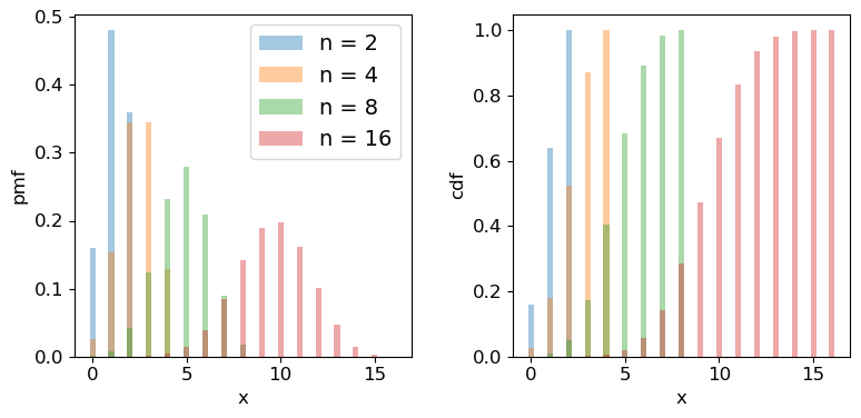
Scipy has the binomial distribution, binom in its stats module. Different properties of the distribution can be accessed via appending the appropriate method to the function call, e.g. sps.binom.pmf, or sps.binom.cdf. Below we plot the pmf and cdf of the distribution for different numbers of trials \(n\). It is formally correct to plot discrete distributions using separated bars, to indicate single discrete values, rather than bins over multiple or continuous values, but sometimes stepped line plots (or even histograms) can be clearer, provided you explain what they show.

## Define theta
theta = 0.6
## Plot as a bar plot
fig, (ax1, ax2) = plt.subplots(1,2, figsize=(9,4))
fig.subplots_adjust(wspace=0.3)
for n in [2,4,8,16]:
    x = np.arange(0,n+1)
    ## Plot the pmf
    ax1.bar(x, sps.binom.pmf(x,n,p=theta), width=0.3, alpha=0.4, label='n = '+str(n))
    ## and the cumulative distribution function:
    ax2.bar(x, sps.binom.cdf(x,n,p=theta), width=0.3, alpha=0.4, label='n = '+str(n))
for ax in (ax1,ax2):
    ax.tick_params(labelsize=12)
    ax.set_xlabel("x", fontsize=12)
    ax.tick_params(axis='x', labelsize=12)
    ax.tick_params(axis='y', labelsize=12)
ax1.set_ylabel("pmf", fontsize=12)
ax2.set_ylabel("cdf", fontsize=12)
ax1.legend(fontsize=14)
plt.show()

Programming example: how many observations do I need?

Imagine that you are developing a research project to study the radio-emitting counterparts of binary neutron star mergers that are detected by a gravitational wave detector. Due to relativistic beaming effects however, radio counterparts are not always detectable (they may be beamed away from us). You know from previous observations and theory that the probability of detecting a radio counterpart from a binary neutron star merger detected by gravitational waves is 0.72. For simplicity you can assume that you know from the gravitational wave signal whether the merger is a binary neutron star system or not, with no false positives.

You need to request a set of observations in advance from a sensitive radio telescope to try to detect the counterparts for each binary merger detected in gravitational waves. You need 10 successful detections of radio emission in different mergers, in order to test a hypothesis about the origin of the radio emission. Observing time is expensive however, so you need to minimise the number of observations of different binary neutron star mergers requested, while maintaining a good chance of success. What is the minimum number of observations of different mergers that you need to request, in order to have a better than 95% chance of being able to test your hypothesis?

(Note: all the numbers here are hypothetical, and are intended just to make an interesting problem!)

Hint

We would like to know the chance of getting at least 10 detections, but the cdf is defined as \(F(x) = P(X\leq x)\). So it would be more useful (and more accurate than calculating 1-cdf for cases with cdf\(\rightarrow 1\)) to use the survival function method (sps.binom.sf).

Solution

We want to know the number of trials \(n\) for which we have a 95% probability of getting at least 10 detections. Remember that the cdf is defined as \(F(x) = P(X\leq x)\), so we need to use the survival function (1-cdf) but for \(x=9\), so that we calculate what we need, which is \(P(X\geq 10)\). We also need to step over increasing values of \(n\) to find the smallest value for which our survival function exceeds 0.95. We will look at the range \(n=\)10-25 (there is no point in going below 10!).

theta = 0.72
for n in range(10,26):
    print("For",n,"observations, chance of 10 or more detections =",sps.binom.sf(9,n,p=theta))

For 10 observations, chance of 10 or more detections = 0.03743906242624486
For 11 observations, chance of 10 or more detections = 0.14226843721973037
For 12 observations, chance of 10 or more detections = 0.3037056744016985
For 13 observations, chance of 10 or more detections = 0.48451538004550243
For 14 observations, chance of 10 or more detections = 0.649052212181364
For 15 observations, chance of 10 or more detections = 0.7780490885758796
For 16 observations, chance of 10 or more detections = 0.8683469020520406
For 17 observations, chance of 10 or more detections = 0.9261375026767835
For 18 observations, chance of 10 or more detections = 0.9605229100485057
For 19 observations, chance of 10 or more detections = 0.9797787381766699
For 20 observations, chance of 10 or more detections = 0.9900228387408534
For 21 observations, chance of 10 or more detections = 0.9952380172098922
For 22 observations, chance of 10 or more detections = 0.9977934546597212
For 23 observations, chance of 10 or more detections = 0.9990043388667172
For 24 observations, chance of 10 or more detections = 0.9995613456019353
For 25 observations, chance of 10 or more detections = 0.999810884619313

So we conclude that we need 18 observations of different binary neutron star mergers, to get a better than 95% chance of obtaining 10 radio detections.

Probability distributions: Poisson

Imagine that we are running a particle detection experiment, e.g. to detect radioactive decays. The particles are detected at random intervals such that the expected mean rate per time interval (i.e. defined over an infinite number of intervals) is \(\lambda\). To work out the distribution of the number of particles \(x\) detected in the time interval, we can imagine splitting the interval into \(n\) equal sub-intervals. Then, if the expected rate \(\lambda\) is constant and the detections are independent of one another, the probability of a detection in any given time interval is the same: \(\lambda/n\). We can think of the sub-intervals as a set of \(n\) repeated Bernoulli trials, so that the number of particles detected in the overall time-interval follows a binomial distribution with \(\theta = \lambda/n\):

In reality the distribution of possible arrival times in an interval is continuous and so we should make the sub-intervals infinitesimally small, otherwise the number of possible detections would be artificially limited to the finite and arbitrary number of sub-intervals. If we take the limit \(n\rightarrow \infty\) we obtain the follow useful results:

\(\frac{n!}{(n-x)!} = \prod\limits_{i=0}^{x-1} (n-i) \rightarrow n^{x}\) and \(\lim\limits_{n\rightarrow \infty} (1-\lambda/n)^{n-x} = e^{-\lambda}\)

where the second limit arises from the result that \(e^{x} = \lim\limits_{n\rightarrow \infty} (1+x/n)^{n}\). Substituting these terms into the expression from the binomial distribution we obtain:

This is the Poisson distribution, one of the most important distributions in observational science, because it describes counting statistics, i.e. the distribution of the numbers of counts in bins. For example, although we formally derived it here as being the distribution of the number of counts in a fixed interval with mean rate \(\lambda\) (known as a rate parameter), the interval can refer to any kind of binning of counts where individual counts are independent and \(\lambda\) gives the expected number of counts in the bin.

For a random variate distributed as a Poisson distribution, \(X\sim \mathrm{Pois}(\lambda)\), \(E[X] = \lambda\) and \(V[X] = \lambda\). The expected variance leads to the expression that the standard deviation of the counts in a bin is equal to \(\sqrt{\lambda}\), i.e. the square root of the expected value. We will see later on that for a Poisson distributed likelihood, the observed number of counts is an estimator for the expected value. From this, we obtain the famous \(\sqrt{counts}\) error due to counting statistics.

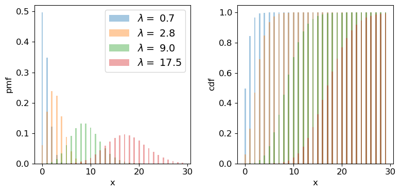
We can plot the Poisson pmf and cdf in a similar way to how we plotted the binomial distribution functions. An important point to bear in mind is that the rate parameter \(\lambda\) does not itself have to be an integer: the underlying rate is likely to be real-valued, but the Poisson distribution produces integer variates drawn from the distribution that is unique to \(\lambda\).

## Plot as a bar plot
fig, (ax1, ax2) = plt.subplots(1,2, figsize=(9,4))
fig.subplots_adjust(wspace=0.3)
## Step through lambda, note that to avoid Python confusion with lambda functions, we make sure we choose
## a different variable name!
for lam in [0.7,2.8,9.0,17.5]:
    x = np.arange(0,30)
    ## Plot the pmf, note that perhaps confusingly, the rate parameter is defined as mu
    ax1.bar(x, sps.poisson.pmf(x,mu=lam), width=0.3, alpha=0.4, label='$\lambda =$ '+str(lam))
    ## and the cumulative distribution function:
    ax2.bar(x, sps.poisson.cdf(x,mu=lam), width=0.3, alpha=0.4, label='$\lambda =$ '+str(lam))
for ax in (ax1,ax2):
    ax.tick_params(labelsize=12)
    ax.set_xlabel("x", fontsize=12)
    ax.tick_params(axis='x', labelsize=12)
    ax.tick_params(axis='y', labelsize=12)
ax1.set_ylabel("pmf", fontsize=12)
ax2.set_ylabel("cdf", fontsize=12)
ax1.legend(fontsize=14)
plt.show()

Programming example: how long until the data are complete?

Following your successful proposal for observing time, you’ve been awarded 18 radio observations of neutron star binary mergers (detected via gravitational wave emission) in order to search for radio emitting counterparts. The expected detection rate for gravitational wave events from binary neutron star mergers is 9.5 per year. Assume that you require all 18 observations to complete your proposed research. According to the time award rules for so-called ‘Target of opportunity (ToO)’ observations like this, you will need to resubmit your proposal if it isn’t completed within 3 years. What is the probability that you will need to resubmit your proposal?

Solution

Since binary mergers are independent random events and their mean detection rate (at least for a fixed detector sensitivity and on the time-scale of the experiment!) should be constant in time, the number of merger events in a fixed time interval should follow a Poisson distribution.

Given that we require the full 18 observations, the proposal will need to be resubmitted if there are fewer than 18 gravitational wave events (from binary neutron stars) in 3 years. For this we can use the cdf, remember again that for the cdf \(F(x) = P(X\leq x)\), so we need the cdf for 17 events. The interval we are considering is 3 years not 1 year, so we should multiply the annual detection rate by 3 to get the correct \(\lambda\):

lam = 9.5*3
print("Probability that < 18 observations have been carried out in 3 years =",sps.poisson.cdf(17,lam))

Probability that < 18 observations have been carried out in 3 years = 0.014388006538141204

So there is only a 1.4% chance that we will need to resubmit our proposal.

Test yourself: is this a surprising detection?

Meanwhile, one of your colleagues is part of a team using a sensitive neutrino detector to search for bursts of neutrinos associated with neutron star mergers detected from gravitational wave events. The detector has a constant background rate of 0.03 count/s. In a 1 s interval following a gravitational wave event, the detector detects a two neutrinos. Without using Python (i.e. by hand, with a calculator), calculate the probability that you would detect less than two neutrinos in that 1 s interval. Assuming that the neutrinos are background detections, should you be suprised about your detection of two neutrinos?

Solution

The probability that you would detect less than two neutrinos is equal to the summed probability that you would detect 0 or 1 neutrino (note that we can sum their probabilities because they are mutually exclusive outcomes). Assuming these are background detections, the rate parameter is given by the background rate \(\lambda=0.03\). Applying the Poisson distribution formula (assuming the random Poisson variable \(x\) is the number of background detections \(N_{\nu}\)) we obtain:

\(P(N_{\nu}<2)=P(N_{\nu}=0)+P(N_{\nu}=1)=\frac{0.03^{0}e^{-0.03}}{0!}+\frac{0.03^{1}e^{-0.03}}{1!}=(1+0.03)e^{-0.03}=0.99956\) to 5 significant figures.

We should be surprised if the detections are just due to the background, because the chance we would see 2 (or more) background neutrinos in the 1-second interval after the GW event is less than one in two thousand! Having answered the question ‘the slow way’, you can also check your result for the probability using the scipy.stats Poisson cdf for \(x=1\).

Note that it is crucial here that the neutrinos arrive within 1 s of the GW event. This is because GW events are rare and the background rate is low enough that it would be unusual to see two background neutrinos appear within 1 s of the rare event which triggers our search. If we had seen two neutrinos only within 100 s of the GW event, we would be much less surprised (the rate expected is 3 count/100 s). We will consider these points in more detail in a later episode, after we have discussed Bayes’ theorem.

Generating random variates drawn from discrete probability distributions

So far we have discussed random variables in an abstract sense, in terms of the population, i.e. the continuous probability distribution. But real data is in the form of samples: individual measurements or collections of measurements, so we can get a lot more insight if we can generate ‘fake’ samples from a given distribution.

The scipy.stats distribution functions have a method rvs for generating random variates that are drawn from the distribution (with the given parameter values). You can either freeze the distribution or specify the parameters when you call it. The number of variates generated is set by the size argument and the results are returned to a numpy array. The default seed is the system seed, but if you initialise your own generator (e.g. using rng = np.random.default_rng()) you can pass this to the rvs method using the random_state parameter.

# Generate 10 variates from Binom(10,0.4)
bn_vars = print(sps.binom.rvs(n=4,p=0.4,size=10))
print("Binomial variates generated:",bn_vars)

# Generate 10 variates from Pois(2.7)
pois_vars = sps.poisson.rvs(mu=2.7,size=10)
print("Poisson variates generated:",pois_vars)

Binomial variates generated: [1 2 0 2 3 2 2 1 2 3]
Poisson variates generated: [6 4 2 2 5 2 2 0 3 5]

Remember that these numbers depend on the starting seed which is almost certainly unique to your computer (unless you pre-select it by passing a bit generator initialised by a specific seed as the argument for the random_state parameter). They will also change each time you run the code cell.

How random number generation works

Random number generators use algorithms which are strictly pseudo-random since (at least until quantum-computers become mainstream) no algorithm can produce genuinely random numbers. However, the non-randomness of the algorithms that exist is impossible to detect, even in very large samples.

For any distribution, the starting point is to generate uniform random variates in the interval \([0,1]\) (often the interval is half-open \([0,1)\), i.e. exactly 1 is excluded). \(U(0,1)\) is the same distribution as the distribution of percentiles - a fixed range quantile has the same probability of occurring wherever it is in the distribution, i.e. the range 0.9-0.91 has the same probability of occuring as 0.14-0.15. This means that by drawing a \(U(0,1)\) random variate to generate a quantile and putting that in the ppf of the distribution of choice, the generator can produce random variates from that distribution. All this work is done ‘under the hood’ within the scipy.stats distribution function.

It’s important to bear in mind that random variates work by starting from a ‘seed’ (usually an integer) and then each call to the function will generate a new (pseudo-)independent variate but the sequence of variates is replicated if you start with the same seed. However, seeds are generated by starting from a system seed set using random and continuously updated data in a special file in your computer, so they will differ each time you run the code.

Key Points

• Probability can be thought of in terms of hypothetical frequencies of outcomes over an infinite number of trials (Frequentist), or as a belief in the likelihood of a given outcome (Bayesian).

• A sample space contains all possible mutually exclusive outcomes of an experiment or trial.

• Discrete probability distributions map a sample space of discrete outcomes (categorical or numerical) on to their probabilities.

• By assigning an outcome to an ordered sequence of integers corresponding to the discrete variates, functional forms for probability distributions (the pmf or probability mass function) can be defined.

• Random variables are drawn from probability distributions. The expectation value (arithmetic mean for an infinite number of sampled variates) is equal to the mean of the distribution function (pmf or pdf).

• The expectation of the variance of a random variable is equal to the expectation of the squared variable minus the squared expectation of the variable.

• Sums of scaled random variables have expectation values equal to the sum of scaled expectations of the individual variables, and variances equal to the sum of scaled individual variances.

• Bernoulli trials correspond to a single binary outcome (success/fail) while the number of successes in repeated Bernoulli trials is given by the binomial distribution.

• The Poisson distribution can be derived as a limiting case of the binomial distribution and corresponds to the probability of obtaining a certain number of counts in a fixed interval, from a random process with a constant rate.

• Random variates can be sampled from Scipy probability distributions using the .rvs method.

• The probability distribution of numbers of objects for a given bin/classification depends on whether the original sample size was fixed at a pre-determined value or not.