8. Conditional probability and joint probability distributions

Overview

Teaching: 60 min
Exercises: 60 min

Questions

• How do we calculate with probabilities, taking account of whether some event is dependent on the occurrence of another?

• How do we define and describe the joint probability distributions of two or more random variables?

Objectives

• Learn the definitions of conditional probability and independence.

• Learn how to use the probability calculus to calculate the probabilities of events or combinations of events, which may be conditional on each other.

• Learn how the pdf and cdf are defined for joint bivariate probability distributions and how to plot them using 3-D and contour plots.

• Learn how the univariate probability distribution for each variable can be obtained from the joint probability distribution by marginalisation.

• Understand the meaning of the covariance and correlation coefficient between two variables, and how they can be applied to define a multivariate normal distribution in Scipy.

In this episode we will be using numpy, as well as matplotlib’s plotting library. Scipy contains an extensive range of distributions in its ‘scipy.stats’ module, so we will also need to import it. Remember: scipy modules should be installed separately as required - they cannot be called if only scipy is imported.

import numpy as np
import matplotlib.pyplot as plt
import scipy.stats as sps

Conditional probability

Consider two events \(A\) and \(B\), whose probability is conditional on one another. I.e. the chance of one event occurring is dependent on whether the other event also occurs. The occurrence of conditional events can be represented by Venn diagrams where the entire area of the diagram represents the sample space of all possible events (i.e. probability \(P(\Omega)=1\)) and the probability of a given event or combination of events is represented by its area on the diagram. The diagram below shows four of the possible combinations of events, where the area highlighted in orange shows the event (or combination) being described in the notation below.

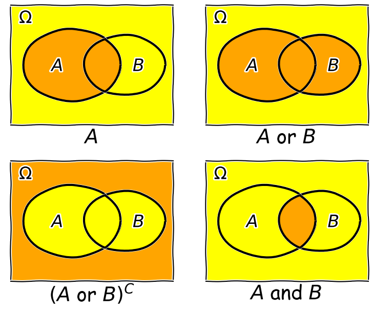
We’ll now decribe these combinations and do the equivalent calculation for the coin flip case where event \(A=\{HH, HT\}\) and event \(B=\{HH, TT\}\) (the probabilities are equal to 0.5 for these two events, so the example diagram is not to scale).

1. Event \(A\) occurs (regardless of whether \(B\) also occurs), with probability \(P(A)\) given by the area of the enclosed shape relative to the total area.
2. Event \((A \mbox{ or } B)\) occurs (in set notation this is the union of sets, \(A \cup B\)). Note that the formal ‘\(\mbox{or}\)’ here is the same as in programming logic, i.e. it corresponds to ‘either or both’ events occurring. The total probability is not \(P(A)+P(B)\) however, because that would double-count the intersecting region. In fact you can see from the diagram that \(P(A \mbox{ or } B) = P(A)+P(B)-P(A \mbox{ and } B)\). Note that if \(P(A \mbox{ or } B) = P(A)+P(B)\) we say that the two events are mutually exclusive (since \(P(A \mbox{ and } B)=0\)).
3. Event \((A \mbox{ or } B)^{C}\) occurs and is the complement of \((A \mbox{ or } B)\) which is everything excluding \((A \mbox{ or } B)\), i.e. \(\mbox{not }(A \mbox{ or } B)\).
4. Event \((A \mbox{ and } B)\) occurs (in set notation this is the intersection of sets, \(A\cap B\)). The probability of \((A \mbox{ and } B)\) corresponds to the area of the overlapping region.

Now in our coin flip example, we know the total sample space is \(\Omega = \{HH, HT, TH, TT\}\) and for a fair coin each of the four outcomes \(X\), has a probability \(P(X)=0.25\). Therefore:

1. \(A\) consists of 2 outcomes, so \(P(A) = 0.5\)
2. \((A \mbox{ or } B)\) consists of 3 outcomes (since \(TH\) is not included), \(P(A \mbox{ or } B) = 0.75\)
3. \((A \mbox{ or } B)^{C}\) corresponds to \(\{TH\}\) only, so \(P(A \mbox{ or } B)^{C}=0.25\)
4. \((A \mbox{ and } B)\) corresponds to the overlap of the two sets, i.e. \(HH\), so \(P(A \mbox{ and } B)=0.25\).

We can also ask the question, what is the probability that an event \(A\) occurs if we know that the other event \(B\) occurs? We write this as the probability of \(A\) conditional on \(B\), i.e. \(P(A\vert B)\). We often also state this is the ‘probability of A given B’.

To calculate this, we can see from the Venn diagram that if \(B\) occurs (i.e. we now have \(P(B)=1\)), the probability of \(A\) also occurring is equal to the fraction of the area of \(B\) covered by \(A\). I.e. in the case where outcomes have equal probability, it is the fraction of outcomes in set \(B\) which are also contained in set \(A\).

This gives us the equation for conditional probability:

So, for our coin flip example, \(P(A\vert B) = 0.25/0.5 = 0.5\). This makes sense because only one of the two outcomes in \(B\) (\(HH\)) is contained in \(A\).

In our simple coin flip example, the sets \(A\) and \(B\) contain an equal number of equal-probability outcomes, and the symmetry of the situation means that \(P(B\vert A)=P(A\vert B)\). However, this is not normally the case.

For example, consider the set \(A\) of people taking this class, and the set of all students \(B\). Clearly the probability of someone being a student, given that they are taking this class, is very high, but the probability of someone taking this class, given that they are a student, is not. In general \(P(B\vert A)\neq P(A\vert B)\).

Note that events \(A\) and \(B\) are independent if \(P(A\vert B) = P(A) \Rightarrow P(A \mbox{ and } B) = P(A)P(B)\). The latter equation is the one for calculating combined probabilities of events that many people are familiar with, but it only holds if the events are independent! For example, the probability that you ate a cheese sandwich for lunch is (generally) independent of the probability that you flip two heads in a row. Clearly, independent events do not belong on the same Venn diagram since they have no relation to one another! However, if you are flipping the coin in order to narrow down what sandwich filling to use, the coin flip and sandwich choice can be classed as outcomes on the same Venn diagram and their combination can become an event with an associated probability.

Test yourself: conditional probability for a dice roll

Use the solution to the dice question above to calculate:

1. The probability of rolling doubles given that the total rolled is greater than 8.
2. The probability of rolling a total greater than 8, given that you rolled doubles.

Solution

1. \(P(B\vert A) = \frac{P(B \mbox{ and } A)}{P(A)}\) (note that the names of the events are arbitrary so we can simply swap them around!). Since \(P(B \mbox{ and } A)=P(A \mbox{ and } B)\) we have \(P(B\vert A) =(2/36)/(10/36)=1/5\).
2. \(P(A\vert B) = \frac{P(A \mbox{ and } B)}{P(B)}\) so we have \(P(A\vert B)=(2/36)/(6/36)=1/3\).

Rules of probability calculus 2

We can now write down the rules of probability calculus and their extensions:

• The convexity rule sets some defining limits: \(0 \leq P(A\vert B) \leq 1 \mbox{ and } P(A\vert A)=1\)
• The addition rule: \(P(A \mbox{ or } B) = P(A)+P(B)-P(A \mbox{ and } B)\)
• The multiplication rule is derived from the equation for conditional probability: \(P(A \mbox{ and } B) = P(A\vert B) P(B)\)

\(A\) and \(B\) are independent if \(P(A\vert B) = P(A) \Rightarrow P(A \mbox{ and } B) = P(A)P(B)\).

We can also ‘extend the conversation’ to consider the probability of \(B\) in terms of probabilities with \(A\):

\[\begin{align} P(B) & = P\left((B \mbox{ and } A) \mbox{ or } (B \mbox{ and } A^{C})\right) \\ & = P(B \mbox{ and } A) + P(B \mbox{ and } A^{C}) \\ & = P(B\vert A)P(A)+P(B\vert A^{C})P(A^{C}) \end{align}\]

The 2nd line comes from applying the addition rule and because the events \((B \mbox{ and } A)\) and \((B \mbox{ and } A^{C})\) are mutually exclusive. The final result then follows from applying the multiplication rule.

Finally we can use the ‘extension of the conversation’ rule to derive the law of total probability. Consider a set of all possible mutually exclusive events \(\Omega = \{A_{1},A_{2},...A_{n}\}\), we can start with the first two steps of the extension to the conversion, then express the results using sums of probabilities:

\[P(B) = P(B \mbox{ and } \Omega) = P(B \mbox{ and } A_{1}) + P(B \mbox{ and } A_{2})+...P(B \mbox{ and } A_{n})\] \[= \sum\limits_{i=1}^{n} P(B \mbox{ and } A_{i})\] \[= \sum\limits_{i=1}^{n} P(B\vert A_{i}) P(A_{i})\]

This summation to eliminate the conditional terms is called marginalisation. We can say that we obtain the marginal distribution of \(B\) by marginalising over \(A\) (\(A\) is ‘marginalised out’).

Test yourself: conditional probabilities and GW counterparts

You are an astronomer who is looking for radio counterparts of binary neutron star mergers that are detected via gravitational wave events. Assume that there are three types of binary merger: binary neutron stars (\(NN\)), binary black holes (\(BB\)) and neutron-star-black-hole binaries (\(NB\)). For a hypothetical gravitational wave detector, the probabilities for a detected event to correspond to \(NN\), \(BB\), \(NB\) are 0.05, 0.75, 0.2 respectively. Radio emission is detected only from mergers involving a neutron star, with probabilities 0.72 and 0.2 respectively.

Assume that you follow up a gravitational wave event with a radio observation, without knowing what type of event you are looking at. Using \(D\) to denote radio detection, express each probability given above as a conditional probability (e.g. \(P(D\vert NN)\)), or otherwise (e.g. \(P(BB)\)). Then use the rules of probability calculus (or their extensions) to calculate the probability that you will detect a radio counterpart.

Solution

We first write down all the probabilities and the terms they correspond to. First the radio detections, which we denote using \(D\):

\(P(D\vert NN) = 0.72\), \(P(D\vert NB) = 0.2\), \(P(D\vert BB) = 0\)

and: \(P(NN)=0.05\), \(P(NB) = 0.2\), \(P(BB)=0.75\)

We need to obtain the probability of a detection, regardless of the type of merger, i.e. we need \(P(D)\). However, since the probabilities of a radio detection are conditional on the merger type, we need to marginalise over the different merger types, i.e.:

\(P(D) = P(D\vert NN)P(NN) + P(D\vert NB)P(NB) + P(D\vert BB)P(BB)\) \(= (0.72\times 0.05) + (0.2\times 0.2) + 0 = 0.076\)

You may be able to do this simple calculation without explicitly using the law of total probability, by using the ‘intuitive’ probability calculation approach that you may have learned in the past. However, learning to write down the probability terms, and use the probability calculus, will help you to think systematically about these kinds of problems, and solve more difficult ones (e.g. using Bayes theorem, which we will come to later).

Joint probability distributions

So far we have considered probability distributions that describe the probability of sampling a single variable. These are known as univariate probability distributions. Now we will consider joint probability distributions which describe the probability of sampling a given combination of multiple variables, where we must make use of our understanding of conditional probability. Such distributions can be multivariate, considering multiple variables, but for simplicity we will focus on the bivariate case, with only two variables \(x\) and \(y.\)

Now consider that each variable is sampled by measurement, to return variates \(X\) and \(Y\). Any combination of variates can be considered as an event, with probability given by \(P(X \mbox{ and } Y)\). For discrete variables, we can simply write the joint probability mass function as:

and so the equivalent for the cdf is:

For continuous variables we need to consider the joint probability over an infinitesimal range in \(x\) and \(y\). The joint probability density function for jointly sampling variates with values \(X\) and \(Y\) is defined as:

I.e. this is the probability that a given measurement of two variables finds them both in the ranges \(x \leq X \leq x+\delta x\), \(y \leq Y \leq y+\delta y\). For the cdf we have:

where \(x'\) and \(y'\) are dummy variables.

In general the probability of variates \(X\) and \(Y\) having values in some region \(R\) is:

Conditional probability and marginalisation

Let’s now recall the multiplication rule of probability calculus for the variates \(X\) and \(Y\) occuring together:

I.e. we can understand the joint probability \(p(x,y)\) in terms of the probability for a particular \(x\) to occur given that a particular \(y\) also occurs. The probability for a given pair of \(x\) and \(y\) is the same whether we consider \(x\) or \(y\) as the conditional variable. We can then write the multiplication rule as:

From this we have the law of total probability:

i.e. we marginalise over \(y\) to find the marginal pdf of \(x\), giving the distribution of \(x\) only.

We can also use the equation for conditional probability to obtain the probability for \(x\) conditional on the variable \(y\) taking on a fixed value (e.g. a drawn variate \(Y\)) equal to \(y_{0}\):

Note that we obtain the probability density \(p(y_{0})\) by integrating the joint probability over \(x\).

Bivariate probability distributions can be visualised using 3-D plots (where the height of the surface shown by the ‘wireframe’ shows the joint probability density) or contour plots (where contours show lines of equal joint probability density). The figures below show the same probability distribution plotted in this way, where the distribution shown is a bivariate normal distribution. Besides showing the joint probability distributions, the figures also show, as black and red solid curves on the side panels, the univariate marginal distributions which correspond to the probability distribution for each (\(x\) and \(y\)) variable, marginalised over the other variable.

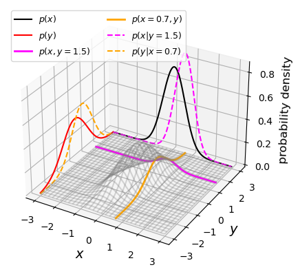
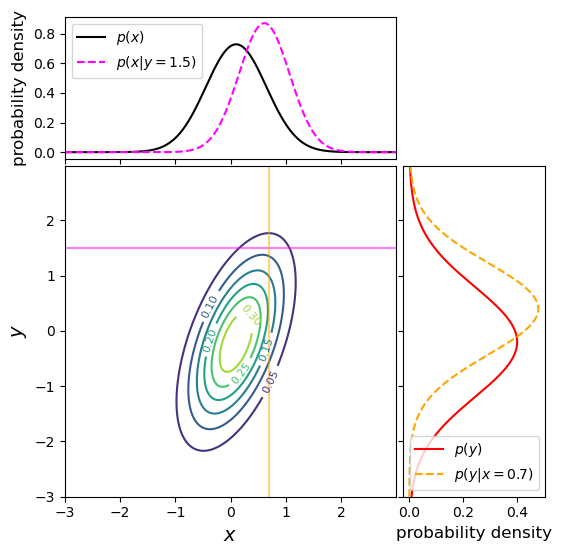
The two coloured (orange and magenta) lines or curves plotted on the joint probability distributions shown above each show a ‘slice’ through the joint distribution which corresponds to the conditional joint probability density at a fixed value of \(y\) or \(x\) (i.e. they correspond to the cases \(p(x\vert y_{0})\) and \(p(y\vert x_{0})\)). The dashed lines with the same colours on the side panels show the univariate probability distributions corresponding to these conditional probability densities. They have the same shape as the joint probability density but are correctly normalised, so that the integrated probability is 1. Since the \(x\) and \(y\) variables are covariant (correlated) with one another (see below), the position of the conditional distribution changes according to the fixed value \(x_{0}\) or \(y_{0}\), so the centre of the curves do not match the centres of the marginal distributions. The curves of conditional probability are also narrower than those of the marginal distributions, since the covariance between \(x\) and \(y\) also broadens both marginal distributions, but not the conditional probability distributions, which correspond to a fixed value on one axis so the covariance does not come into play.

Properties of bivariate distributions: mean, variance, covariance

We can use our result for the marginal pdf to derive the mean and variance of variates of one variable that are drawn from a bivariate joint probability distribution. Here we quote the results for \(x\), but the results are interchangeable with the other variable, \(y\).

Firstly, the expectation (mean) is given by:

I.e. we first marginalise (integrate) the joint distribution over the variable \(y\) to obtain \(p(x)\), and then the mean is calculated in the usual way. Note that since the distribution is bivariate we use the subscript \(x\) to denote which variable we are quoting the mean for.

The same procedure is used for the variance:

So far, we have only considered how to convert a bivariate joint probability distribution into the univariate distribution for one of its variables, i.e. by marginalising over the other variable. But joint distributions also have a special property which is linked to the conditional relationship between its variables. This is known as the covariance

The covariance of variates \(X\) and \(Y\) is given by:

We can obtain the term \(E[XY]\) by using the joint distribution:

In the case where \(X\) and \(Y\) are independent variables, \(p(x\vert y)=p(x)\) and we obtain:

I.e. for independent variables the covariance \(\sigma_{xy}=0\). The covariance is a measure of how dependent two variables are on one another, in terms of their linear correlation. An important mathematical result known as the Cauchy-Schwarz inequality implies that \(\lvert \mathrm{Cov}(X,Y)\rvert \leq \sqrt{V[X]V[Y]}\). This means that we can define a correlation coefficient which measures the degree of linear dependence between the two variables:

where \(-1\leq \rho(X,Y) \leq 1\). Note that variables with positive (non-zero) \(\rho\) are known as correlated variables, while variables with negative \(\rho\) are anticorrelated. For independent variables the correlation coefficient is clearly zero, but it is important to note that the covariance (and hence the correlation coefficient) can also be zero for non-independent variables. E.g. consider the relation between random variate \(X\) and the variate \(Y\) calculated directly from \(X\), \(Y=X^{2}\), for \(X\sim U[-1,1]\):

The covariance (and correlation) is zero even though the variables \(X\) and \(Y\) are completely dependent on one another. This result arises because the covariance measures the linear relationship between two variables, but if the relationship between two variables is non-linear, it can result in a low (or zero) covariance and correlation coefficient.

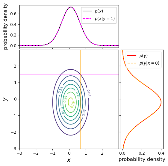
An example of a joint probability density for two independent variables is shown below, along with the marginal distributions and conditional probability distributions. This distribution uses the same means and variances as the covariant case shown above, but covariance between \(x\) and \(y\) is set to zero. We can immediately see that the marginal and conditional probability distributions (which have the same fixed values of \(x_{0}\) and \(y_{0}\) as in the covariant example above) are identical for each variable. This is as expected for independent variables, where \(p(x)=p(x\vert y)\) and vice versa.

Finally we note that these approaches can be generalised to multivariate joint probability distributions, by marginalising over multiple variables. Since the covariance can be obtained between any pair of variables, it is common to define a covariance matrix, e.g.:

The diagonal elements correspond to the variances of each variable (since the covariance of a variable with itself is simply the variance), while off-diagonal elements correspond to the covariance between pairs of variables. Note that in terms of numerical values, the matrix is symmetric about the diagonal, since by definition \(\sigma_{xy}=\sigma_{yx}\).

Programming example: plotting joint probability distributions

It is useful to be able to plot bivariate pdfs and their marginal and conditional pdfs yourself, so that you can develop more intuition for how conditional probability works, e.g. by changing the covariance matrix of the distribution. We made the plots above using the following code, first to generate the pdfs:

import scipy.integrate as spint
# Freeze the parameters of the bivariate normal distribution: means and covariance matrix for x and y
bvn = sps.multivariate_normal([0.1, -0.2], [[0.3, 0.3], [0.3, 1.0]])
# Next we must set up a grid of x and y values to calculate the bivariate normal for, on each axis the
# grid ranges from -3 to 3, with step size 0.01
x, y = np.mgrid[-3:3:0.01, -3:3:0.01]
xypos = np.dstack((x, y))
# Calculate the bivariate joint pdf and for each variable marginalise (integrate) the joint pdf over the 
# other variable to obtain marginal pdfs for x and y
xypdf = bvn.pdf(xypos)
xpdf = spint.simpson(xypdf,y,axis=1)
ypdf = spint.simpson(xypdf,x,axis=0)
# Now define x and y ranges to calculate a 'slice' of the joint pdf, corresponding to the conditional pdfs
# for given x_0 and y_0
xrange = np.arange(-3,3,0.01)
yrange = np.arange(-3,3,0.01)
# We must create corresponding ranges of fixed x and y
xfix = np.full(len(yrange),0.7)
yfix = np.full(len(xrange),1.5)
# And define our arrays for the pdf to be calculated
xfix_pos = np.dstack((xfix, yrange))
yfix_pos = np.dstack((xrange, yfix))
# Now we calculate the conditional pdfs for each case, remembering to normalise by the integral of the 
# conditional pdf so the integrated probability = 1
bvny_xfix = bvn.pdf(xfix_pos)/spint.simpson(bvn.pdf(xfix_pos),yrange)
bvnx_yfix = bvn.pdf(yfix_pos)/spint.simpson(bvn.pdf(yfix_pos),xrange)

Next we made the 3D plot as follows. You should run the iPython magic command %matplotlib notebook somewhere in your notebook (e.g. in the first cell, with the import commands) in order to make the plot interactive, which allows you to rotate it with the mouse cursor and really benefit from the 3-D plotting style.

fig = plt.figure()
ax = fig.add_subplot(projection='3d')
# Plot the marginal pdfs on the sides of the 3D box (corresponding to y=3 and x=-3)
ax.plot3D(x[:,0],np.full(len(xpdf),3.0),xpdf,color='black',label=r'$p(x)$')
ax.plot3D(np.full(len(ypdf),-3.0),y[0,:],ypdf,color='red',label=r'$p(y)$')
# Plot the slices through the joint pdf corresponding to the conditional pdfs:
ax.plot3D(xrange,yfix,bvn.pdf(yfix_pos),color='magenta',linewidth=2,label=r'$p(x,y=1.5)$')
ax.plot3D(xfix,yrange,bvn.pdf(xfix_pos),color='orange',linewidth=2,label=r'$p(x=0.7,y)$')
# Plot the normalised conditional pdf on the same box-sides as the marginal pdfs
ax.plot3D(xrange,np.full(len(xrange),3.0),bvnx_yfix,color='magenta',linestyle='dashed',label=r'$p(x\vert y=1.5)$')
ax.plot3D(np.full(len(yrange),-3.0),yrange,bvny_xfix,color='orange',linestyle='dashed',label=r'$p(y\vert x=0.7)$')
# Plot the joint pdf as a wireframe:
ax.plot_wireframe(x, y, xypdf, rstride=20, cstride=20, alpha=0.3, color='gray')
# Plot labels and the legend
ax.set_xlabel(r'$x$',fontsize=14)
ax.set_ylabel(r'$y$',fontsize=14)
ax.set_zlabel(r'probability density',fontsize=12)
ax.legend(fontsize=9,ncol=2)
plt.show()

Look at the online documentation for the scipy.stats.multivariate_normal function to find out what the parameters do. Change the covariance and variance values to see what happens to the joint pdf and the marginal and conditional pdfs. Remember that the variances correspond to diagonal elements of the covariance matrix, i..e to the elements [0,0] and [1,1] of the array with the covariance matrix values. The amount of diagonal ‘tilt’ of the joint pdf will depend on the magnitude of the covariant elements compared to the variances. You should also bear in mind that since the integration is numerical, based on the calculated joint pdf values, the marginal and conditional pdfs will lose accuracy if your joint pdf contains significant probability outside of the calculated region. You could fix this by e.g. making the calculated region larger, while setting the x and y limits to show the same zoom in of the plot.

We chose plot_wireframe() to show the joint pdf, so that the other pdfs (and the slices through the joint pdf to show the conditional pdfs), are easily visible. But you could use other versions of the 3D surface plot such as plot_surface() also including a colour map and colour bar if you wish. If you use a coloured surface plot you can set the transparency (alpha) to be less than one, in order to see through the joint pdf surface more easily.

Finally, if you want to make a traditional contour plot, you could use the following code:

# We set the figsize so that we get a square plot with x and y axes units having equal dimension 
# (so the contours are not artificially stretched)
fig = plt.figure(figsize=(6,6))
# Add a gridspec with two rows and two columns and a ratio of 3 to 7 between
# the size of the marginal axes and the main axes in both directions.
# We also adjust the subplot parameters to obtain a square plot.
gs = fig.add_gridspec(2, 2,  width_ratios=(7, 3), height_ratios=(3, 7), left=0.1, right=0.9, 
                          bottom=0.1, top=0.9, wspace=0.03, hspace=0.03)
# Set up the subplots and their shared axes
ax = fig.add_subplot(gs[1, 0])
ax_xpdfs = fig.add_subplot(gs[0, 0], sharex=ax)
ax_ypdfs = fig.add_subplot(gs[1, 1], sharey=ax)
# Turn off the tickmark values where necessary
ax_xpdfs.tick_params(axis="x", labelbottom=False)
ax_ypdfs.tick_params(axis="y", labelleft=False)
con = ax.contour(x, y, xypdf)  # The contour plot
# Marginal and conditional pdfs plotted in the side/top panel
ax_xpdfs.plot(x[:,0],xpdf,color='black',label=r'$p(x)$')
ax_ypdfs.plot(ypdf,y[0,:],color='red',label=r'$p(y)$')
ax_xpdfs.plot(xrange,bvnx_yfix,color='magenta',linestyle='dashed',label=r'$p(x\vert y=1.5)$')
ax_ypdfs.plot(bvny_xfix,yrange,color='orange',linestyle='dashed',label=r'$p(y\vert x=0.7)$')
# Lines on the contour show the slices used for the conditional pdfs
ax.axhline(1.5,color='magenta',alpha=0.5)
ax.axvline(0.7,color='orange',alpha=0.5)
# Plot labels and legend
ax.set_xlabel(r'$x$',fontsize=14)
ax.set_ylabel(r'$y$',fontsize=14)
ax_xpdfs.set_ylabel(r'probability density',fontsize=12)
ax_ypdfs.set_xlabel(r'probability density',fontsize=12)
ax.clabel(con, inline=1, fontsize=8) # This adds labels to show the value of each contour level
ax_xpdfs.legend()
ax_ypdfs.legend()
#plt.savefig('2d_joint_prob.png',bbox_inches='tight')
plt.show()

Probability distributions: multivariate normal

scipy.stats contains a number of multivariate probability distributions, with the most commonly used being multivariate_normal considered above, which models the multivariate normal pdf:

where bold symbols denote vectors and matrices: \(\mathbf{x}\) is a real \(k\)-dimensional column vector of variables \([x_{1}\,x_{2}\, ...\,x_{k}]^{\mathrm{T}}\), \(\boldsymbol{\mu} = \left[E[X_{1}]\,E[X_{2}]\,...\,E[X_{k}]\right]^{\mathrm{T}}\) and \(\mathbf{\Sigma}\) is the \(k\times k\) covariance matrix of elements:

Note that \(\mathrm{T}\) denotes the transpose of the vector (to convert a row-vector to a column-vector and vice versa) while \(\lvert\mathbf{\Sigma}\rvert\) and \(\mathbf{\Sigma}^{-1}\) are the determinant and inverse of the covariance matrix respectively. A single sampling of the distribution produces variates \(\mathbf{X}=[X_{1}\,X_{2}\, ...\,X_{k}]^{\mathrm{T}}\) and we describe their distribution with \(\mathbf{X} \sim N_{k}(\boldsymbol{\mu},\mathbf{\Sigma})\).

Scipy’s multivariate_normal comes with the usual pdf and cdf methods although its general functionality is more limited than for the univariate distributions. Examples of the pdf plotted for a bivariate normal are given above for the 3D and contour plotting examples. The rvs method can also be used to generate random data drawn from a multivariate distribution, which can be especially useful when simulating data with correlated (but normally distributed) errors, provided that the covariance matrix of the data is known.

Programming example: multivariate normal random variates

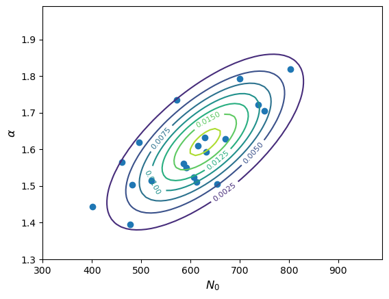
You are simulating measurements of a sample of gamma-ray spectra which are described by a power-law model, at energy \(E\) (in GeV) the photon flux density (in photons/GeV) is given by \(N(E)=N_{0}E^{-\alpha}\) where \(N_{0}\) is the flux density at 1 GeV. Based on the statistical errors in the expected data, you calculate that your measured values of \(N_{0}\) and \(\alpha\) should be covariant with means \(\mu_{N_{0}}=630\), \(\mu_{\alpha}=1.62\), standard deviations \(\sigma_{N_{0}}=100\), \(\sigma_{\alpha}=0.12\) and covariance \(\sigma_{N_{0}\alpha}=8.3\). Assuming that the paired measurements of \(N_{0}\) and \(\alpha\) are drawn from a bivariate normal distribution, simulate a set of 20 measured pairs of these quantities and plot them as a scatter diagram, along with the confidence contours of the underlying distribution.

Solution

# Set up the parameters:
means = [630, 1.62]
sigmas = [100, 0.12]
covar = 8.3
# Freeze the distribution:
bvn = sps.multivariate_normal(means, [[sigmas[0]**2, covar], [covar, sigmas[1]**2]])
# Next we must set up a grid of x and y values to calculate the bivariate normal for. We choose a range that
# covers roughly 3-sigma around the means
N0_grid, alpha_grid = np.mgrid[300:1000:10, 1.3:2.0:0.01]
xypos = np.dstack((N0_grid, alpha_grid))
# Make a random set of 20 measurements. For reproducibility we set a seed first:
rng = np.random.default_rng(38700)
xyvals = bvn.rvs(size=20, random_state=rng)
# The output is an array of shape (20,2), for clarity we will assign each column to the corresponding variable:
N0_vals = xyvals[:,0]
alpha_vals = xyvals[:,1]
# Now make the plot
plt.figure()
con = plt.contour(N0_grid, alpha_grid, bvn.pdf(xypos))
plt.scatter(N0_vals, alpha_vals)
plt.xlabel(r'$N_{0}$',fontsize=12)
plt.ylabel(r'$\alpha$',fontsize=12)
plt.clabel(con, inline=1, fontsize=8)
plt.show()

Simulating correlated data from mathematical and physical models

Many measurements will result in simultaneous data for multiple variables which will often be correlated, and many physical situations will also naturally produce correlations between random variables. E.g. the temperature of a star depends on its surface area and luminosity, which both depend on the mass, metallicity and stellar age (and corresponding stage in the stellar life-cycle). Such variables are often easier to relate using mathematical models with one or more variables being drawn independently from appropriate statistical distributions, and the correlations between them being produced by their mathematical relationship. In general, the resulting distributions will not be multivariate normal, unless they are related to multivariate normal variates by simple linear transformations.

Programming example: calculating fluxes from power-law spectra

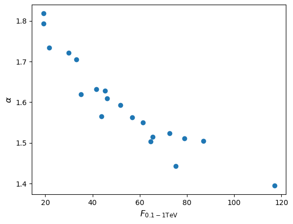
Now imagine you want to use your measurements of gamma ray spectra from the previous programming example, to predict the integrated photon flux \(F_{\rm 0.1-1 TeV}\) in the energy range \(10^{2}\)-\(10^{3}\) GeV. Starting from your simulated measurements of \(N_{0}\) and \(\alpha\), make a scatter plot of the photon flux in this range vs. the index \(\alpha\). Does the joint probability distribution of \(\alpha\) and \(F_{\rm 0.1-1 TeV}\) remain a multivariate normal? Check your answer by repeating the simulation for \(10^{6}\) measurements of \(N_{0}\) and \(\alpha\) and also plotting a histogram of the calculated fluxes.

Hint

The integrated photon flux is equal to \(\int^{1000}_{100} N_{0} E^{-\alpha}\mathrm{d}E\)

Solution

The integrated photon flux is \(\int^{1000}_{100} N_{0} E^{-\alpha}\mathrm{d}E = \frac{N_{0}}{1-\alpha}\left(1000^{(1-\alpha)}-100^{(1-\alpha)}\right)\). We can apply this to our simulated data:

flux_vals = (N0_vals/(1-alpha_vals))*(1000**(1-alpha_vals)-100**(1-alpha_vals))
plt.figure()
plt.scatter(flux_vals, alpha_vals)
plt.xlabel(r'$F_{\rm 0.1-1 TeV}$',fontsize=12)
plt.ylabel(r'$\alpha$',fontsize=12)
plt.show()

Since a power-law (i.e. non-linear) transformation is applied to the measurements we would not expect the flux distribution to remain normal, although the joint distribution of \(\alpha\) (i.e. marginalised over flux) should of course remain normal. Repeating the simulation for a million pairs of \(N_{0}\) and \(\alpha\) we obtain (setting marker size s=0.01 for the scatter plot and using bins=1000 and density=True for the histogram):

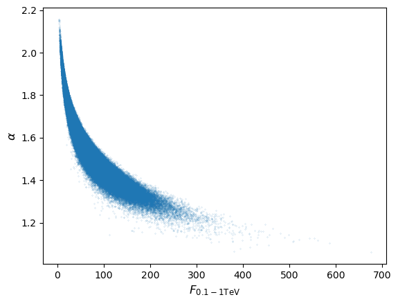
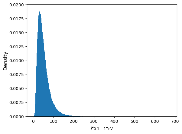
As expected, the flux distribution is clearly not normally distributed, it is positively skewed to high fluxes, resulting in the curvature of the joint distribution.

Sums of multivariate random variables and the multivariate Central Limit Theorem

Consider two \(m\)-dimensional multivariate random variates, \(\mathbf{X}=[X_{1}, X_{2},..., X_{m}]\) and \(\mathbf{Y}=[Y_{1}, Y_{2},..., Y_{m}]\), which are drawn from different distributions with mean vectors \(\boldsymbol{\mu}_{x}\), \(\boldsymbol{\mu}_{y}\) and covariance matrices \(\boldsymbol{\Sigma}_{x}\), \(\boldsymbol{\Sigma}_{y}\). The sum of these variates, \(\mathbf{Z}=\mathbf{X}+\mathbf{Y}\) follows a multivariate distribution with mean \(\boldsymbol{\mu}_{z}=\boldsymbol{\mu}_{x}+\boldsymbol{\mu}_{y}\) and covariance \(\boldsymbol{\Sigma}_{z}=\boldsymbol{\Sigma}_{x}+\boldsymbol{\Sigma}_{y}\). I.e. analogous to the univariate case, the result of summing variates drawn from multivariate distributions is to produce a variate with mean vector equal to the sum of the mean vectors and covariance matrix equal to the sum of the covariance matrices.

The analogy with univariate distributions also extends to the Central Limit Theorem, so that the sum of \(n\) random variates drawn from multivariate distributions, \(\mathbf{Y}=\sum\limits_{i=1}^{n} \mathbf{X}_{i}\) is drawn from a distribution which for large \(n\) becomes asymptotically multivariate normal, with mean vector equal to the sum of mean vectors and covariance matrix equal to the sum of covariance matrices. This also means that for averages of \(n\) random variates drawn from multivariate distributions \(\bar{\mathbf{X}} = \frac{1}{n} \sum\limits_{i=1}^{n} \mathbf{X}_{i}\), the mean vector is equal to the average of mean vectors while the covariance matrix is equal to the sum of covariance matrices divided by \(n^{2}\):

Key Points

• Events consist of sets of outcomes which may overlap, leading to conditional dependence of the occurrence of one event on another. The conditional dependence of events can be described graphically using Venn diagrams.

• The probability of an event A occurring, given that B occurs, is in general not equal to the probability of B occurring, given that A occurs.

• Calculations with conditional probabilities can be made using the probability calculus, including the addition rule, multiplication rule and extensions such as the law of total probability.

• Joint probability distributions show the joint probability of two or more variables occuring with given values.

• The univariate pdf of one of the variables can be obtained by marginalising (integrating) the joint pdf over the other variable(s).

• If the probability of a variable taking on a value is conditional on the value of the other variable (i.e. the variables are not independent), the joint pdf will appear tilted.

• The covariance describes the linear relationship between two variables, when normalised by their standard deviations it gives the correlation coefficient between the variables.

• Zero covariance and correlation coefficient arises when the two variables are independent and may also occur when the variables are non-linearly related.

• The covariance matrix gives the covariances between different variables as off-diagonal elements, with their variances given along the diagonal of the matrix.

• The distributions of sums of multivariate random variates have vectors of means and covariance matrices equal to the sum of the vectors of means and covariance matrices of the individual distributions.

• The sums of multivariate random variates also follow the (multivariate) central limit theorem, asymptotically following multivariate normal distributions for sums of large samples.