Array Calculations with Numpy

Overview

Teaching: 20 min
Exercises: 30 min

Questions

• How can I perform calculations on large arrays quickly, using numpy functions?

Objectives

• Use the library of numpy functions for fast array calculations.

• Understand how arrays of different shapes can be operated on using broadcasting.

• Mask arrays to hide unwanted data and use masked array ufuncs to operate on them.

• Write functions to perform complex operations on arrays.

Numpy offers an enormous range of pre-compiled functions in its numerical libraries, which allow a wide range of tasks to be completed on large arrays of data with speeds comparable to or approaching those of dedicated compiler languages such as Fortran or C++. We describe some examples of some of these functions here, but you should read the Numpy documentation online to find many more. A good general rule is that if you can think of a numerical method or function that you want to use, it is already implemented in numpy (or possibly scipy). So googling what you want to do together with the terms numpy or scipy is a good way to find what you need.

More on Numpy Ufuncs

Numpy ufuncs are pre-compiled (usually in C) functions that that operate on ndarray type objects (i.e. numpy arrays). They operate element-wise (item by item) on the array and support type casting (python will try to make non matching data types work) and broadcasting (i.e. python will try to make different array shapes work, see below). Most mathematical functions are available (we include some examples in this Episode and elsewhere in this lesson) and it’s also possible to write your own.

Ufuncs which operate on arrays come in two main flavours: unary ufuncs operate on a single array, while binary ufuncs operate on a pair of arrays. An example of binary ufuncs are the standard mathematical operators, which are wrappers for the underlying numpy functions:

import numpy as np

a = np.linspace(10,50,5)
b = np.arange(5)
print("a =",a)
print("b =",b,"\n")

print("a + b =",a+b,"is the same as np.add(a,b) =",np.add(a,b))
print("a - b =",a-b,"is the same as np.subtract(a,b) =",np.subtract(a,b))
print("-a =",-a,"is the same as np.negative(a) =",np.negative(a))
print("a * b =",a*b,"is the same as np.multiply(a,b)=",np.multiply(a,b))
print("a / b =",a/b,"is the same as np.divide(a,b)=",np.divide(a,b))
print("a // b =",a//b,"is the same as np.floor_divide(a,b)=",np.floor_divide(a,b))
print("a**b =",a**b,"is the same as np.power(a,b)=",np.power(a,b))
print("a % b =",a%b,"is the same as np.mod(a,b)=",np.mod(a,b))

a = [10. 20. 30. 40. 50.]
b = [0 1 2 3 4] 

a + b = [10. 21. 32. 43. 54.] is the same as np.add(a,b) = [10. 21. 32. 43. 54.]
a - b = [10. 19. 28. 37. 46.] is the same as np.subtract(a,b) = [10. 19. 28. 37. 46.]
-a = [-10. -20. -30. -40. -50.] is the same as np.negative(a) = [-10. -20. -30. -40. -50.]
a * b = [  0.  20.  60. 120. 200.] is the same as np.multiply(a,b)= [  0.  20.  60. 120. 200.]
a / b = [        inf 20.         15.         13.33333333 12.5       ] is the same as np.divide(a,b)= [        inf 20.         15.         13.33333333 12.5       ]
a // b = [nan 20. 15. 13. 12.] is the same as np.floor_divide(a,b)= [nan 20. 15. 13. 12.]
a**b = [1.00e+00 2.00e+01 9.00e+02 6.40e+04 6.25e+06] is the same as np.power(a,b)= [1.00e+00 2.00e+01 9.00e+02 6.40e+04 6.25e+06]
a % b = [nan  0.  0.  1.  2.] is the same as np.mod(a,b)= [nan  0.  0.  1.  2.]

Writing these operations using the common mathematical operators is quicker than using the full numpy function names - and they follow the usual mathematical rules for order of operation, with powers calculated first, then division and multiplication then addition and subtraction. But you should remember that these are array operations and not operations on single variables!

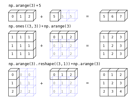
Broadcasting

Binary ufuncs operate on two arrays (e.g. addition or multiplication of two arrays, to give a simple example). If the arrays have the same shape (same number of dimensions, each with the same size) the operation is applied to the corresponding pairs of elements in the array (i.e. the pair of elements with the same indices).

However, a great advantage of numpy’s arrays and ufuncs is that they allow broadcasting. Numpy’s broadcasting rules allow binary ufuncs to be applied to arrays of different shapes, provided that the shape of the smaller array can be mapped on to the same shape as the larger array in an unambiguous way. The broadcasting rules can be simplified to:

1. If both arrays have a different number of dimensions, the shape of the one with fewer dimensions is padded (on the left side of the shape tuple) with dimensions of size 1 so that the dimensions are now matched.

2. If the shapes are not the same in any dimension, the array with size 1 in that dimension is extended in size (repeating the same values), to match the other array.

3. However, if the sizes in a given dimension don’t match and neither is equal to 1 an error is raised.

The figure below (created using the code here) shows examples of successful broadcasting.

Challenge

Write a function that can take an input array of dates expressed with integer type as YYYYMMDD (e.g. 19950325, as read in by genfromtxt from the KNMI data set) and returns three separate arrays of year, month and the day of the month. To calculate these quantities you should use only the numpy functions corresponding to standard mathematical operations with math symbol wrappers (see above).

Hint

To get you started, this is how you can find the year: year = date // 10**4

Solution

def get_ymd(date):
    '''Takes as input the date as integer type YYYYMMDD and returns year, month 
    (as integer 1-12) and day of the month'''

    year = date // 10**4
    month = date // 10**2 % 100
    day = date % 100

    return year, month, day

Common mathematical functions

Besides the common mathematical operators, there are ufuncs for all of the common mathematical functions. E.g.:

print("Square root of a:",np.sqrt(a))
print("Exponential of b:",np.exp(b))
print("log_10(a) =",np.log10(a)) # Log in base 10
print("ln(a) =",np.log(a)) # Natural log
print("log_2(a) =",np.log2(a)) # Log in base 2
print("\n\n")
      
angles = np.linspace(0.,2*np.pi,10) # Pi can be called with np.pi
print("Angles in radians:",angles)
print("Angles in degrees:",np.degrees(angles)) # To go from degrees to radians, use np.radians

print("tan(b): ",np.tan(a)) # Functions include inverse (arctan etc.) and other trig functions

Square root of a: [3.16227766 4.47213595 5.47722558 6.32455532 7.07106781]
Exponential of b: [ 1.          2.71828183  7.3890561  20.08553692 54.59815003]
log_10(a) = [1.         1.30103    1.47712125 1.60205999 1.69897   ]
ln(a) = [2.30258509 2.99573227 3.40119738 3.68887945 3.91202301]
log_2(a) = [3.32192809 4.32192809 4.9068906  5.32192809 5.64385619]


Angles in radians: [0.         0.6981317  1.3962634  2.0943951  2.7925268  3.4906585
 4.1887902  4.88692191 5.58505361 6.28318531]
Angles in degrees: [  0.  40.  80. 120. 160. 200. 240. 280. 320. 360.]
tan(b):  [ 0.64836083  2.23716094 -6.4053312  -1.11721493 -0.27190061]

Conditional functions

There are also a large number of useful numpy functions for manipulating and selecting from arrays. For example numpy.where allows the user to set a condition to be applied to each element of the array (given by the first argument), with two different results to be applied, according to whether the condition is satisfied or not (second and third argument respectively). For example, what function would the following code produce?

t = np.linspace(0,10*np.pi,1000)
a = np.sin(t)
b = np.where(a > 0,1,0)

plt.figure()
plt.plot(t,b)
plt.xlabel('t',fontsize=12)
plt.ylabel('b',fontsize=12)
plt.show()

Solution

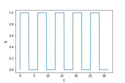
A square wave function!

In this case, constants were given as the results for the True or False cases of the condition, but functions could also be specified instead.

Random numbers and statistics

Numpy’s numerical libraries include a large number of functions that are useful for statistical simulations (e.g. generating random numbers), as well as calculating standard statistical quantities. For example, random numbers can be generated for a large number of simulations using numpy.random and suffixing with the required distribution (and its arguments - see the numpy documentation for details). E.g.:

a = np.random.normal(size=10) # drawn from normal distribution (mean 0, standard deviation 1)
b = np.random.uniform(2,6,size=10) # drawn from uniform distribution with min. 2, max. 6

print("a = ",a,"\n")
print("b =",b)

The random numbers will change every time you generate them, so they won’t match the example values shown below. To prevent this you could fix the random number generating ‘seed’ to the same value each time (e.g. using numpy.random.seed). Fixing random number seeds is generally a bad idea, as you almost always need your generated values to be statistically independent each time.

a =  [-0.30022351 -0.2436521   0.82529598  1.45559054  2.81468678  0.63432945
  0.45292206 -0.7189043  -1.5688999  -2.07679378] 

b = [4.91409402 5.20504639 4.10317644 4.52392586 4.12252377 5.19390016
 2.63697377 2.09074333 5.82355927 5.00880279]

There are a large number of functions to calculate statistical properties of data, e.g.:

mean = np.mean(a)
std_dev = np.std(a,ddof=1)
median = np.median(a)

# For the standard deviation of a sample, the degrees of freedom ddof=1 
print("For a, mean =",np.mean(a),"median =",np.median(a),"and standard deviation =",np.std(a,ddof=1))
print("For b, mean =",np.mean(b),"median =",np.median(b),"and standard deviation =",np.std(b,ddof=1))

# The statistical quantities for a large random sample should be closer to the population ('true') values:
c = np.random.normal(size=100000)
d = np.random.uniform(2,6,size=100000)

print("For c, mean =",np.mean(c),"median =",np.median(c),"and standard deviation =",np.std(c,ddof=1))
print("For d, mean =",np.mean(d),"median =",np.median(d),"and standard deviation =",np.std(d,ddof=1))

For a, mean = 0.1274351220779665 median = 0.10463498050131667 and standard deviation = 1.4379104160216345
For b, mean = 4.36227458161702 median = 4.719009939469249 and standard deviation = 1.1807239934047047
For c, mean = -0.003106470300092659 median = -0.0020945245248079037 and standard deviation = 1.0019999302839593
For d, mean = 4.00191762092067 median = 4.001883767677743 and standard deviation = 1.1542783586377883

For multi-dimensional data sets the default is to flatten the array and calculate a single statistical quantity for all the values, but by specifying the axis as an integer or tuple of integers, quantities can be calculated along specific dimensions of the array. This can be useful if you want to arrange your data into many sub-samples corresponding to, e.g. columns in the array, and calculate separate statistical quantities for each sub-sample. For example:

x = np.linspace(1,6,10)
y = np.random.normal(x,np.sqrt(x),size=(20,10)) # Mean and standard deviation increase with x

y_mean = np.mean(y,axis=0) # Measure mean along each column of 20 values
y_std = np.std(y,axis=0,ddof=1) # Measure standard deviation

print("Means =",y_mean)
print("Standard deviations =",y_std)

Means = [1.10406239 1.79198285 2.41687801 2.61184147 2.37594309 3.46102472 4.72351714 4.66671086 4.68688962 6.8386863 ]
Standard deviations = [1.21478777 1.46095133 1.53221715 1.89578884 1.66559555 2.28753281 1.90451327 2.55568894 2.19337894 2.31425862]

Numpy functions like these can be used to handle data sets, but for more extensive analysis, especially with large and complex data sets Pandas (which is based in large part on numpy and scipy) is a more suitable and versatile library.

Masked Arrays

In some situations your array may contain elements with no data, bad data, or data which you wish to filter from your analysis for some other reason. You can remove this data using a condition to filter out the elements you don’t want, but this only works if the resulting array can be flattened and you don’t need to preserve its shape. However, if you want to keep the shape of your data array (e.g. for statistical calculations along a particular axis), it is useful to create a masked array. These can be created using the numpy.ma module, which also includes equivalents of common numpy functions that can be applied to masked arrays (for which the usual numpy functions will not work).

First, we will add some nan values in random locations in the y array we generated previously:

# First randomly select indices of elements from y to change values to NaN in new array y2
cols = np.random.random_integers(0,9,size=20)
rows = np.random.random_integers(0,19,size=20)
y2 = np.copy(y)
y2[rows,cols] = np.nan

y2_mean = np.mean(y2,axis=0) # Measure mean along each column of 20 values
y2_std = np.std(y2,axis=0,ddof=1) # Measure standard deviation

print("Means =",y2_mean)
print("Standard deviations =",y2_std)

Means = [       nan        nan        nan        nan        nan 3.46102472
        nan        nan        nan        nan]
Standard deviations = [       nan        nan        nan        nan        nan 2.28753281
        nan        nan        nan        nan]

Any columns containing nan will result in nan for the statistics calculated along those columns. We can produce a masked array with nan values masked. One way to create a masked array is to use the masked_array function with a Boolean array of True/False values with the same shape as the array to be masked, e.g.:

y2_ma = np.ma.masked_array(y2,np.isnan(y2))

y2_ma_mean = np.ma.mean(y2_ma,axis=0) # Measure mean along each column of 20 values
y2_ma_std = np.ma.std(y2_ma,axis=0,ddof=1) # Measure standard deviation

print("Means =",y2_ma_mean)
print("Standard deviations =",y2_ma_std)

Means = [0.8922926559222217 1.679217577416684 2.432410192332734 2.5727061459634673
 2.2115371803066557 3.4610247170590283 4.475816052299866 4.786879589526783
 4.743040460933355 6.887791934103876]
Standard deviations = [1.1636287759233295 1.5121734615501945 1.6169210355493306
 1.974709637455112 1.5354844835950414 2.2875328102951253
 1.8266358576564314 2.5670126872971335 2.236916568224871
 2.3669453874421658]

We must be careful with any statistical measures from masked data, in case the missing values cause the measurements to be biased in some way.

Using Numpy to calculate with the KNMI data

Now we can use the methods we have looked at above to quickly calculate monthly quantities from the KNMI meteorological data, and plot them. First, read in the data (substituting missing values with -9999:

data = np.genfromtxt('KNMI_20200825.txt',delimiter=',',comments='#',skip_header=97,names=True,dtype=None,filling_values=-9999)

Challenge Part 1

For the first part of the challenge, write a function which takes as input the structured data array read in above, the station number and the name of the variable you want to plot (you can see the variable names using print data.dtype to show the field information for the structured array). The function should select only the dates and the variable values for that station and when the quantity corresponding to that variable was measured (see the solution to the Challenge at the end of the previous Episode).

Next, the function should recalculate the dates as arrays of integer type for the day, month and year (see the Challenge earlier in this Episode), and assign the values of the variable to a 3-D array, where the axes of the array correspond to year (measured since the first year when data was taken), month and day of the month. Before assigning values to the array, create your array so that it is already filled with nan values, to identify positions in the array that correspond to dates with no data for that variable, or which do not correspond to real dates (such as Feb 31).

Finally, your function should output the resulting 3-D array as well as the integer value of the first year in the return data array, so that year values corresponding to that axis can be determined (the days and months should be self-evident from the indices).

If you find this part too difficult or time consuming, you can look at the solution and skip ahead to the next part. This first part is really focussed on array manipulation using the principles discussed in the previous Episode. The second part focusses on using methods discussed in this Episode.

Part 1 Solution

def get_3d_data(data,stn_num,varname):
    '''Read in structured data array, station number (int) and variable name (str),
    select data for that station and variable only, and then assign the data to a 
    3D array where axes correspond to the year, month and day. 
    Output: 3D data array and the starting year for the data'''

    # First select date and variable values for given station number
    data_stn = data[data['STN'] == stn_num] # Select data for that station only
    data_stn = data_stn[data_stn[varname] != -9999] # Only include data when the 
    selected variable was measured
    year, month, day = get_dmy(data_stn['YYYYMMDD'])
    variable =  data_stn[varname]

    # Now lets define a 3D array for our variable, where each axis corresponds to a 
    year, month and day. 
    # First, set the dimensions:

    y_len = (year[-1]-year[0])+1  # This assumes years are in chronological order
    m_len = 12  # 12 months in a year...
    d_len = 31 # Allow up to 31, excess days are filled with NaN and we should filter 
    them in calculations

    # Set up the 3D array:
    data_array = np.full((y_len,m_len,d_len),np.nan)

    # Now fill the 3D array with the corresponding data values.
    # indices start at 0 so days/months should be shifted back by 1
    data_array[year-year[0],month-1,day-1] = variable

    return data_array, year[0]

Challenge Part 2

Now write a function that does the following:

• Takes as input the original structured array produced by genfromtxt from the KNMI data file, a station number and a list of variable names
• Looping through the list of variable names, then within the loop:
  1. Create a 3-D data array using the function written in Part 1 of this Challenge.
  2. Create a masked version of the 3-D array to ignore the elements with nan.
  3. Use the masked array to calculate the mean values for the 12 months in the year (i.e. averaging the data over all years and days in that month)
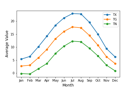
  4. Plot the means vs. month, so that all the variables in the list are plotted in the same plot (use plt.show() outside the loop at the end of the function). For extra brownie points, add a legend which shows the variable names vs. plot symbol/colour (depending on the type of plot) and correct by a factor 10 the variables that are given in tenths of a unit, to show them in the normal units.

Use your function to plot the monthly average of the daily minimum (TN), mean (TG) and maximum (TX) temperatures for a selected station.

Hint

To plot a legend you can include an argument label in the plotting function call (e.g. plt.plot), where the value of label is a string, and then include the function plt.legend() before plotting.

Part 2 Solution

def plot_monthly_allyears(data,stn_num,var_list):
    '''Read in the structured data array of KNMI data, station number and list of variables.
    
    Loops through the list of variables to obtain a 3-D (year,month,day) array for that variable,
    masks the array to ignore missing data and calculate the means (over all years) for each month.
    Then plot the variable so all appear on the same plot. 

    Does not return anything.'''

    months = ['Jan','Feb','Mar','Apr','May','Jun','Jul','Aug','Sep','Oct','Nov','Dec']
    plt.figure()
    for i, varname in enumerate(var_list):
        # Make 3D array for that variable
        data_array, year_start = get_3d_data(data,stn_num,varname)
        # Create a masked array to remove nan values
        data_array_ma = np.ma.masked_array(data_array,np.isnan(data_array))
        if (varname[0] in ('D','U','Q','V') or varname[-1] == 'H' or varname == 'SP'):
        # Find the mean value for each month by averaging over all years and days in that month
        means = np.ma.mean(data_array_ma,axis=(0,2))
        else:
        means = 0.1*np.ma.mean(data_array_ma,axis=(0,2))
        plt.plot(np.arange(1,13),means,label=varname,marker='o',linewidth=2,linestyle='-')
    # These plot commands apply to the whole plot so we can end the loop here
    plt.xticks(np.arange(1,13),months)
    plt.ylabel("Average Value",fontsize=12)
    plt.xlabel("Month",fontsize=12)
    plt.legend()
    plt.show()
    return

Now let’s plot the temperatures for Eindhoven:

plot_monthly_allyears(data,370,['TX','TG','TN'])  

Key Points

• Numpy ufuncs operate element-wise (item by item) on an array.

• Common mathematical operators applied to numpy arrays act as wrappers for fast array calculations.

• Binary ufuncs operate on two arrays: if the arrays have different shapes which are compatible, the operation uses broadcasting rules.

• Many operations and numerical methods (such as random number generation) can be carried out with numpy functions.

• Arrays can be masked to allow unwanted elements (e.g. with nan values) to be ignored in array calculations using special masked array ufuncs.

• Define your own functions that carry out complex array operations by combining different numpy functions.