Numerical Methods with Scipy

Overview

Teaching: 40 min
Exercises: 0 min

Questions

• What numerical methods are available in the Scipy library?

Objectives

• Discover the wide range of numerical methods that are available in Scipy sub-packages

• See how some of the subpackages can be used for interpolation, integration, model fitting and Fourier analysis of time-series.

Introducing Scipy

Scipy is a collection of packages and functions based on numpy, with a goal of performing scientific computation with numerical methods which have similar functionality as common numerical languages such as MATLAB, IDL and R. The scipy library is heavily integrated with numpy and matplotlib.

Scipy is organised into sub-packages covering different topics - you need to import them individually. The sub-packages are:

We’ll look at some examples here, but the sub-package topics will give you an idea of where to look for things online, by looking at their documentation. Also, as with numpy, you can usually find what you want by combining what you want to do with the names ‘scipy’, ‘numpy’ (or just ‘Python’) in a google search. The trick is figuring out the formal way to describe what it is that you are trying to do (although a verbal description of it will sometimes work!).

Check the function documentation!

It is very important that you always check the documentation for a scipy (or numpy) function before using it for the first time. This is not only to see what inputs the function requires (and what its outputs are), but also to check the assumptions that go into the function calculation (e.g. the curve_fit function require errors on the data to be normally distributed). You should never use a function as a ‘black box’ without understanding the basics of what it is supposed to do and what special conditions are required for the results to make sense.

For the functions described below, as you go through them take a look at the documentation (google the function name and ‘scipy’ but be sure to look at the latest version, or the one suitable for your installation of scipy). You will see that many functions have a lot of other capabilities, including a variety of additional arguments to control how they work, and sometimes additional methods that make them more versatile.

Interpolation

With the interpolation sub-package you can carry out 1-D interpolation using a variety of techniques (e.g. linear, cubic), taking as input 1-D arrays of \(x\) and \(y\) values and a set of new \(x\) values, for which the interpolated \(y\) values should be determined:

import numpy as np
import matplotlib.pyplot as plt
%matplotlib inline

from scipy.interpolate import interp1d

x = np.linspace(0, 10, num=11, endpoint=True)
y = np.cos(-x**2/9.0)
f = interp1d(x, y)
f2 = interp1d(x, y, kind='cubic')
f3 = interp1d(x, y, kind='nearest')

xnew = np.linspace(0, 10, num=100, endpoint=True)

plt.figure()
plt.plot(x, y, '-o')
plt.plot(xnew, f(xnew), '-') 
plt.plot(xnew, f2(xnew), '--')
plt.plot(xnew, f3(xnew), ':')
plt.plot(x, y, '-o')
plt.xlabel('x',fontsize=14)
plt.ylabel('y',fontsize=14)
plt.tick_params(axis='both', labelsize=12)
plt.legend(['data','linear','cubic','nearest'], loc='best',fontsize=14)
plt.savefig('interpolation.png')
plt.show()

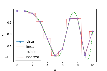
A variety of 1- and N-dimensional interpolation functions are also available.

Integration

Within scipy.integrate, the quad function is useful for evaluating the integral of a given function, e.g. suppose we want to integrate any function \(f(x)\) within the boundaries \(a\) and \(b\): \(\int_{a}^{b} f(x) dx\)

As a specific example let’s try \(\int_{0}^{\pi/2} sin(x) dx\), which we know must be exactly 1:

from scipy.integrate import quad

# quad integrates the function using adaptive Gaussian quadrature from the Fortran QUADPACK library

result, error = quad(np.sin, 0, np.pi/2)

print("Integral =",result)
print("Error =",error)

Besides the result, the function also estimates a numerical error (which arises due to the floating point accuracy, i.e. number of bits used for numbers, in the calculations).

Integral = 0.9999999999999999
Error = 1.1102230246251564e-14

Optimization and model-fitting

The scipy.optimize sub-package contains a large number of functions for optimization, i.e. solving an equation to maximize or minimize (the more common situation) the result. These methods are particularly useful for model-fitting, when we want to minimize the difference between a set of model predictions and the data itself. To use these fully use these methods, accounting for statistical errors, you should study statistical methods and data analysis, which is beyond the scope of this course. For now, we introduce a few of these methods as a primer with a few simple use cases.

First we’re going to generate a sine wave time series, adding scatter to the data points with random numbers drawn from a normal distribution:

from scipy import optimize

x_data = np.linspace(-5, 5, num=50)
y_data = 2.9 * np.sin(1.5 * x_data) + np.random.normal(size=50)

# We know that the data lies on a sine wave, but not the amplitudes or the period.

plt.plot(x_data,y_data,"o")
plt.figure()
plt.plot(x_data,y_data,"o")
plt.xlabel('x',fontsize=14)
plt.ylabel('y',fontsize=14)
plt.show()

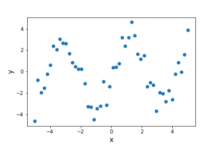
The scatter in the data means that the parameters of the sine-wave cannot be easily determined from the data itself. A standard approach is to minimise the squared residuals (the residual is the difference, data - model). Under certain conditions (if the errors are normally distributed), this least squares minimization can be done using scipy.optimize’s curve_fit function.

First, we need to define the function we want to fit to the data:

# Set up a function with free parameters to fit to the data

def test_func(x, a, b):
    return a * np.sin(b * x)

Now we call curve_fit, giving as arguments our function name, the data \(x\) and \(y\) values, and the starting parameters for the model (given as a list or array). If no error bars on the data points are specified, curve_fit will return the best-fitting model parameters which minimize the squared residuals, which we can also use to plot the best-fitting model together with the data. We will not consider the case where error bars are specified (which minimizes the so-called chi-squared statistic) or the parameter covariance which is also produced as output (and which can be used to estimate model parameter). These should be discussed in any course on statistical methods.

params, params_covariance = optimize.curve_fit(test_func, x_data, y_data, p0=[2, 2])
print("Best-fitting parameters = ",params)

plt.figure()
plt.plot(x_data,y_data,"o")
plt.plot(x_data,test_func(x_data,params[0],params[1]),"r")
plt.xlabel('x',fontsize=14)
plt.ylabel('y',fontsize=14)
plt.show()

Best fitting parameters: [2.70855704 1.49003739]

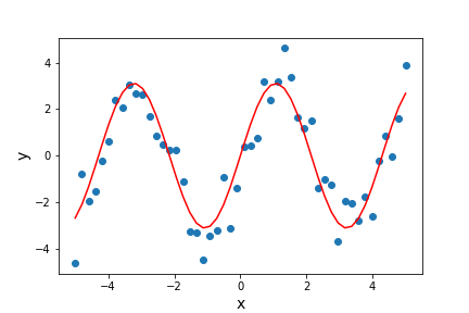
The best-fitting parameters are similar to but not exactly the same as the ones we used to generate the data. This isn’t surprising because the random errors in the data will lead to some uncertainty in the fitted parameter values, which can be estimated using a full statistical treatment of the fit results.

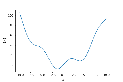
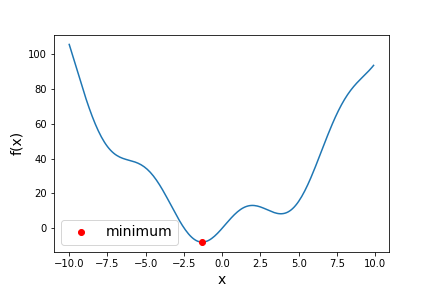
Besides model-fitting, we may want to simply find the minimum of a function (if the maximum is needed, it can usually be found by using minimization with the function to be maximized multiplied by -1!). For example, let’s find the minimum in this function:

def f(x):
    return x**2 + 10*np.sin(x)

x = np.arange(-10, 10, 0.1)

plt.figure()
plt.plot(x, f(x))
plt.xlabel('x',fontsize=14)
plt.ylabel('f(x)',fontsize=14)
plt.show() 

For general cases such as this (where we aren’t dealing with random errors that require minimization of squared residuals), we can use methods provided by the scipy.optimize function minimize. There are a wide range of optimization methods which minimize can use by changing the, from ‘downhill simplex’ (such as Nelder-Mead) to conjugate gradient methods (e.g. BFGS). You should look them up to find out how they work. They all have pros and cons.

result = optimize.minimize(f, x0=0, method='BFGS')

print("Results from the minimization are:",result)

plt.plot(x, f(x))
plt.plot(result.x, f(result.x),"ro",label="minimum")
plt.xlabel('x',fontsize=14)
plt.ylabel('f(x)',fontsize=14)
plt.legend(fontsize=14)
plt.show()

The result obtained by minimize is a compound object that contains all the information of the minimization attempt. result.fun gives the minimum value of the function and result.x gives the best-fitting model parameters corresponding to the function minimum. The other parameters depend on the method used, but may include the Jacobian (1st order partial derivative of the function, evaluated at the minimum) and the Hessian (2nd order partial derivative of the function, evaluated at the minimum) or its inverse (related to the covariance matrix). The use of the 2nd-order derivatives should be considered in any course covering statistical methods applied to data.

     fun: -7.945823375615215
hess_inv: array([[0.08589237]])
     jac: array([-1.1920929e-06])
 message: 'Optimization terminated successfully.'
    nfev: 18
     nit: 5
    njev: 6
  status: 0
 success: True
       x: array([-1.30644012])

Fast Fourier Transforms

Fourier transforms can be used to decompose a complex time-series signal into its component frequencies of variation, which can yield powerful insights into the nature of the variability process, or important astrophysical parameters (such as the rotation period of a neutron star, or the orbital period of a planet or a binary system). Particularly useful are the class of Fast Fourier Transforms (FFT), which use clever numerical methods to reduce the number of operations needed to calculate a Fourier transform of a time-series of length \(n\), from \(n^{2}\) operations to only \(\sim n \ln(n)\).

Scipy’s fft sub-package contains a range of FFT functions for calculating 1-, 2- and N-D FFTs, as well as inverse FFTs. Note that scipy.fft supercedes the former FFT subpackage scipy.fftpack. If you have an older version of Scipy, the code below will not work, but it should work if you change the name of the sub-package to fftpack (or even better, update your version of Scipy!).

First, let’s simulate a sinusoidal signal with a period of 0.5 s, embedded in Gaussian noise:

time_step = 0.02  # 0.02 s time bins
period = 0.5  # 0.5 s period

time = np.arange(0, 20, time_step)
sig = (np.sin(2 * np.pi / period * time) + 2.0 * np.random.randn(time.size))

plt.figure()
plt.plot(time, sig)
plt.xlabel('t (s)',fontsize=14)
plt.ylabel('sig',fontsize=14)
plt.show()

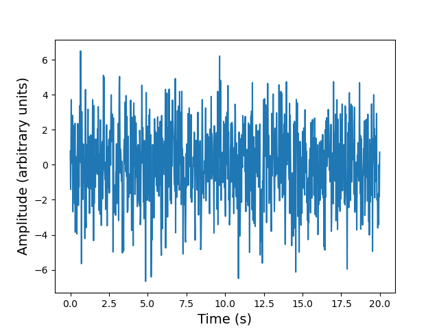
You cannot easily see the 0.5 s period in the light curve (this is also true if you zoom in), due to the large amplitude of noise added to the signal. Instead, let’s calculate the FFT of the signal, and from this measure the power, which is the modulus-squared of the complex amplitude of the FFT, and scales with the variance contributed to the time-series at each frequency. The resulting plot of power vs. frequency is called a power spectrum, also referred to as a periodogram when used to look for periodic signals, which will show up as a peak at a particular frequency.

Formally the scipy 1-D FFT function scipy.fft.fft calculates the so-called Discrete Fourier Transform (DFT) \(y[k]\) of a contiguous time-series (i.e. measurements contained in equal time bins, with one measurement right after another with no gaps between bins).

For a time-series \(x[n]\) of length \(N\), \(y[k]\) is defined as:

where \(k\) denotes the frequency bin (and \(i\) is the imaginary unit). The zero frequency bin has an amplitude equal to the sum over all the \(x[n]\) values. Formally, \(k\) takes both negative and positive values, extending to \(\pm \frac{N}{2}\) (the so-called Nyquist frequency). However, for real-valued time-series the negative frequency values are just the complex conjugates of the corresponding positive-frequency values, so the convention is to only plot the positive frequencies. It’s important to note however that the results of the scipy.fft.fft function are ‘packed’ in the resulting DFT array so that for even \(N\), the elements \(y[1]...y[N/2-1]\) contain the positive frequency terms (in ascending frequency order) while elements \(y[N/2]...y[N-1]\) contain the negative frequency terms (in order of decreasing absolute frequency).

Since the DFT does not take any time units, the actual frequencies \(f[k]\) may be calculated separately (e.g. using the scipy.fft.fftfreq function). They can also be easily calculated by hand, since they are simply related to \(k\) and the duration of the time-series via \(f[k]=k/(N\Delta t)\) where \(\Delta t\) is the time step corresponding to one time-series bin. Thus, the Nyquist frequency corresponds to \(f[N/2] = 1/(2\Delta t)\) and only depends on the bin size.

Now that we know what scipy’s FFT function will give us, let’s calculate it for our noisy sinusoidal signal.

from scipy import fft

# The FFT of the signal
sig_fft = fft.fft(sig)

# And the power (sig_fft is of complex dtype), power is the modulus-squared of the FT
power = np.abs(sig_fft)**2

# The corresponding frequencies
sample_freq = fft.fftfreq(sig.size, d=time_step)

# Plot the FFT power, we only plot +ve frequencies (for real time series, -ve frequencies are 
# complex conjugate of +ve). Note that if we don't restrict the index range to sig.size//2,
# the line plotting the power spectrum will wrap around to the negative value of the Nyquist frequency
plt.figure()
plt.plot(sample_freq[:sig.size//2], power[:sig.size//2])
plt.xlim(0,26.)
plt.xlabel('Frequency [Hz]',fontsize=14)
plt.ylabel('Power',fontsize=14)
plt.show()

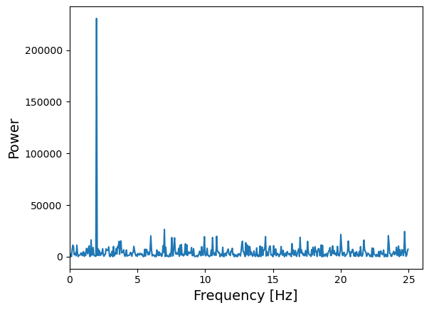
The sinusoidal signal at 2 Hz frequency is very clear in the power spectrum.

fft can also be given a multi-dimensional array as input, so that it will measure multiple FFTs along a given axis (the last axis is used as a default). This can be used when multiple FFTs of equal-length segments of a time-series need to be calculated quickly (instead of repeatedly looping over the fft function).

Besides the FFT functions in scipy, numpy also contains a suite of FFT functions (in numpy.fft). When searching for periodic signals against a background of white noise (random variations which are statistically independent from one to the next), the scipy and numpy functions are useful when the time-series consists of contiguous bins. If there are gaps in the time-series however, the related Lomb-Scargle periodogram can be used. It can be found in Astropy, in the timeseries analysis sub-package, as astropy.timeseries.LombScargle.

Key Points

• Scipy sub-packages need to be individually loaded - import scipy and then referring to the package name is not sufficient. Instead use, e.g. from scipy import fft.

• Specific functions can also be loaded separately such as from scipy.interpolate import interp1d.

• For model fitting when errors are normally distributed you can use scipy.optimize.curve_fit. For more general function minimization use scipy.optimize.minimize

• Be careful with how Scipy’s Fast Fourier Transform results are ordered in the output arrays.

• Always be careful to read the documentation for any Scipy sub-packages and functions to see how they work and what is assumed.