Programming Style
Overview
Teaching: 15 min
Exercises: 15 minQuestions
How can I make my programs more readable?
How do most programmers format their code?
Objectives
Provide sound justifications for basic rules of coding style.
Refactor one-page programs to make them more readable and justify the changes.
Use Python community coding standards (PEP-8).
Coding style
Coding style helps us to understand the code better. It helps to maintain and change the code. Python relies strongly on coding style, as we may notice by the indentation we apply to lines to define different blocks of code. Python proposes a standard style through one of its first Python Enhancement Proposals (PEP), PEP8, and highlight the importance of readability in the Zen of Python.
We highlight some points:
- Document your code
- Use clear, meaningful variable names
- Indents should be with 4 whitespaces, not a tab - note that IDEs and Jupyter notebooks will automatically convert tabs to whitespaces, but check that this is the case!
- Python lines should be shorter than 79 characters
- No deeply indented code
- Variables in small case (
mass = 45) - Global variables in uppercase if your are using them (e.g.
OUTPUT = False) - Avoid builtin names
- Use underscores for readability (
def cal_density():) - Classes (see later) in camel case (
RingedPlanet) - Always avoid commented out code (at least in the final stages of development)
- Use descriptive names for variables (e.g. not
l2 = [])
Follow standard Python style in your code.
- PEP8:
a style guide for Python that discusses topics such as how you should name variables,
how you should use indentation in your code,
how you should structure your
importstatements, etc. Adhering to PEP8 makes it easier for other Python developers to read and understand your code, and to understand what their contributions should look like. The PEP8 application and Python library can check your code for compliance with PEP8. - Google style guide on Python supports the use of PEP8 and extend the coding style to more specific structure of a Python code, which may be interesting also to follow. Google’s formatting application is called “yapf”.
Reminder: use docstrings to provide builtin help.
- If the first thing in a function is a character string that is not assigned directly to a variable, Python attaches it to the function as the builtin help variable.
- Called a docstring (short for “documentation string”).
def average(values):
    "Return average of values, or None if no values are supplied."

    if len(values) == 0:
        return None
    return sum(values) / len(values)

help(average)
Help on function average in module __main__:

average(values)
    Return average of values, or None if no values are supplied.
Multiline Strings
Often use multiline strings for documentation. These start and end with three quote characters (either single or double) and end with three matching characters.
"""This string spans
multiple lines.

Blank lines are allowed."""
What Will Be Shown?
Highlight the lines in the code below that will be available as help. Are there lines that should be made available, but won’t be? Will any lines produce a syntax error or a runtime error?
"Find maximum edit distance between multiple sequences."
# This finds the maximum distance between all sequences.

def overall_max(sequences):
    '''Determine overall maximum edit distance.'''

    highest = 0
    for left in sequences:
        for right in sequences:
            '''Avoid checking sequence against itself.'''
            if left != right:
                this = edit_distance(left, right)
                highest = max(highest, this)

    # Report.
    return highest
Document This
Turn the comment on the following function into a docstring and check that
helpdisplays it properly.def middle(a, b, c): # Return the middle value of three. # Assumes the values can actually be compared. values = [a, b, c] values.sort() return values[1]Solution
def middle(a, b, c):
    '''Return the middle value of three.

    Assumes the values can actually be compared.'''
    values = [a, b, c]
    values.sort()
    return values[1]
Clean Up This Code
- Read this short program and try to predict what it does.
- Run it: how accurate was your prediction?
- Refactor the program to make it more readable. Remember to run it after each change to ensure its behavior hasn’t changed.
- Compare your rewrite with your neighbor’s. What did you do the same? What did you do differently, and why?
n = 10
s = 'et cetera'
print(s)
i = 0
while i < n:
    # print('at', j)
    new = ''
    for j in range(len(s)):
        left = j-1
        right = (j+1)%len(s)
        if s[left]==s[right]: new += '-'
        else: new += '*'
    s=''.join(new)
    print(s)
    i += 1
Solution
Here’s one solution.
def string_machine(input_string, iterations):
    """ Generates iteratively marked strings for the same adjacent characters

    Takes input_string and generates a new string with -'s and *'s
    corresponding to characters that have identical adjacent characters
    or not, respectively.  Iterates through this procedure with the resultant
    strings for the supplied number of iterations.
    """
    print(input_string)
    input_string_length = len(input_string)
    old = input_string
    for i in range(iterations):
        new = ''
        # iterate through characters in previous string
        for j in range(input_string_length):
            left = j-1
            right = (j+1) % input_string_length  # ensure right index wraps around
            if old[left] == old[right]:
                new += '-'
            else:
                new += '*'
        print(new)
        # store new string as old
        old = new

string_machine('et cetera', 10)
et cetera *****-*** ----*-*-- ---*---*- --*-*-*-* **------- ***-----* --**---** *****-*** ----*-*-- ---*---*-
Key Points
Follow standard Python style in your code.
Use docstrings to provide builtin help.
Errors and Exceptions
Overview
Teaching: 30 min
Exercises: 0 minQuestions
How does Python report errors?
How can I handle errors in Python programs?
Objectives
To be able to read a traceback, and determine where the error took place and what type it is.
To be able to describe the types of situations in which syntax errors, indentation errors, name errors, index errors, and missing file errors occur.
Every programmer encounters errors, both those who are just beginning, and those who have been programming for years. Encountering errors and exceptions can be very frustrating at times, and can make coding feel like a hopeless endeavour. However, understanding what the different types of errors are and when you are likely to encounter them can help a lot. Once you know why you get certain types of errors, they become much easier to fix.
Errors in Python have a very specific form, called a traceback. Let’s examine one:
# This code has an intentional error. You can type it directly or
# use it for reference to understand the error message below.
def favorite_ice_cream():
    ice_creams = [
        'chocolate',
        'vanilla',
        'strawberry'
    ]
    print(ice_creams[3])

favorite_ice_cream()
IndexError                                Traceback (most recent call last)
<ipython-input-7-e5b074b4d20d> in <module>
      9     print(ice_creams[3])
     10
---> 11 favorite_ice_cream()

<ipython-input-7-e5b074b4d20d> in favorite_ice_cream()
      7         'strawberry'
      8     ]
----> 9     print(ice_creams[3])
     10
     11 favorite_ice_cream()

IndexError: list index out of range
This particular traceback has two levels. You can determine the number of levels by looking for the number of arrows on the left hand side. In this case:
-
The first shows code from the cell above, with an arrow pointing to Line 8 (which is
favorite_ice_cream()). -
The second shows some code in the function
favorite_ice_cream, with an arrow pointing to Line 6 (which isprint(ice_creams[3])).
The last level is the actual place where the error occurred.
The other level(s) show what function the program executed to get to the next level down.
So, in this case, the program first performed a
function call to the function favorite_ice_cream.
Inside this function,
the program encountered an error on Line 6, when it tried to run the code print(ice_creams[3]).
Long Tracebacks
Sometimes, you might see a traceback that is very long – sometimes they might even be 20 levels deep! This can make it seem like something horrible happened, but the length of the error message does not reflect severity, rather, it indicates that your program called many functions before it encountered the error. Most of the time, the actual place where the error occurred is at the bottom-most level, so you can skip down the traceback to the bottom.
So what error did the program actually encounter?
In the last line of the traceback,
Python helpfully tells us the category or type of error (in this case, it is an IndexError)
and a more detailed error message (in this case, it says “list index out of range”).
If you encounter an error and don’t know what it means, it is still important to read the traceback closely. That way, if you fix the error, but encounter a new one, you can tell that the error changed. Additionally, sometimes knowing where the error occurred is enough to fix it, even if you don’t entirely understand the message.
If you do encounter an error you don’t recognize, try looking at the official documentation on errors. However, note that you may not always be able to find the error there, as it is possible to create custom errors. In that case, hopefully the custom error message is informative enough to help you figure out what went wrong.
Syntax Errors
When you forget a colon at the end of a line,
accidentally add one space too many when indenting under an if statement,
or forget a parenthesis,
you will encounter a syntax error.
This means that Python couldn’t figure out how to read your program.
This is similar to forgetting punctuation in English:
for example,
this text is difficult to read there is no punctuation there is also no capitalization
why is this hard because you have to figure out where each sentence ends
you also have to figure out where each sentence begins
to some extent it might be ambiguous if there should be a sentence break or not
People can typically figure out what is meant by text with no punctuation, but people are much smarter than computers. If Python doesn’t know how to read the program, it will give up and inform you with an error. For example:
def some_function()
    msg = 'hello, world!'
    print(msg)
     return msg
  File "<ipython-input-3-6bb841ea1423>", line 1
    def some_function()
                       ^
SyntaxError: invalid syntax
Here, Python tells us that there is a SyntaxError on line 1,
and even puts a little arrow in the place where there is an issue.
In this case the problem is that the function definition is missing a colon at the end.
Actually, the function above has two issues with syntax.
If we fix the problem with the colon,
we see that there is also an IndentationError,
which means that the lines in the function definition do not all have the same indentation:
def some_function():
    msg = 'hello, world!'
    print(msg)
     return msg
  File "<ipython-input-4-ae290e7659cb>", line 4
    return msg
    ^
IndentationError: unexpected indent
Both SyntaxError and IndentationError indicate a problem with the syntax of your program,
but an IndentationError is more specific:
it always means that there is a problem with how your code is indented.
Tabs and Spaces
Some indentation errors are harder to spot than others. In particular, mixing spaces and tabs can be difficult to spot because they are both whitespace. In the example below, the first two lines in the body of the function
some_functionare indented with tabs, while the third line — with spaces. If you’re working in a Jupyter notebook, be sure to copy and paste this example rather than trying to type it in manually because Jupyter automatically replaces tabs with spaces.def some_function(): msg = 'hello, world!' print(msg) return msgVisually it may be difficult to spot the error (although Jupyter notebooks will now highlight the problem for you). Fortunately, Python does not allow you to mix tabs and spaces.
  File "<ipython-input-5-653b36fbcd41>", line 4
    return msg
              ^
TabError: inconsistent use of tabs and spaces in indentation
Variable Name Errors
Another very common type of error is called a NameError,
and occurs when you try to use a variable that does not exist.
For example:
print(a)
---------------------------------------------------------------------------
NameError                                 Traceback (most recent call last)
<ipython-input-7-9d7b17ad5387> in <module>()
----> 1 print(a)

NameError: name 'a' is not defined
Variable name errors come with some of the most informative error messages, which are usually of the form “name ‘the_variable_name’ is not defined”.
Why does this error message occur? That’s a harder question to answer, because it depends on what your code is supposed to do. However, there are a few very common reasons why you might have an undefined variable. The first is that you meant to use a string, but forgot to put quotes around it:
print(hello)
---------------------------------------------------------------------------
NameError                                 Traceback (most recent call last)
<ipython-input-8-9553ee03b645> in <module>()
----> 1 print(hello)

NameError: name 'hello' is not defined
The second reason is that you might be trying to use a variable that does not yet exist.
In the following example,
count should have been defined (e.g., with count = 0) before the for loop:
for number in range(10):
    count = count + number
print('The count is:', count)
---------------------------------------------------------------------------
NameError                                 Traceback (most recent call last)
<ipython-input-9-dd6a12d7ca5c> in <module>()
      1 for number in range(10):
----> 2     count = count + number
      3 print('The count is:', count)

NameError: name 'count' is not defined
Finally, the third possibility is that you made a typo when you were writing your code.
Let’s say we fixed the error above by adding the line Count = 0 before the for loop.
Frustratingly, this actually does not fix the error.
Remember that variables are case-sensitive,
so the variable count is different from Count. We still get the same error,
because we still have not defined count:
Count = 0
for number in range(10):
    count = count + number
print('The count is:', count)
---------------------------------------------------------------------------
NameError                                 Traceback (most recent call last)
<ipython-input-10-d77d40059aea> in <module>()
      1 Count = 0
      2 for number in range(10):
----> 3     count = count + number
      4 print('The count is:', count)

NameError: name 'count' is not defined
Index Errors
Next up are errors having to do with containers (like lists and strings) and the items within them. If you try to access an item in a list or a string that does not exist, then you will get an error. This makes sense: if you asked someone what day they would like to get coffee, and they answered “caturday”, you might be a bit annoyed. Python gets similarly annoyed if you try to ask it for an item that doesn’t exist:
letters = ['a', 'b', 'c']
print('Letter #1 is', letters[0])
print('Letter #2 is', letters[1])
print('Letter #3 is', letters[2])
print('Letter #4 is', letters[3])
Letter #1 is a
Letter #2 is b
Letter #3 is c
---------------------------------------------------------------------------
IndexError                                Traceback (most recent call last)
<ipython-input-11-d817f55b7d6c> in <module>()
      3 print('Letter #2 is', letters[1])
      4 print('Letter #3 is', letters[2])
----> 5 print('Letter #4 is', letters[3])

IndexError: list index out of range
Here,
Python is telling us that there is an IndexError in our code,
meaning we tried to access a list index that did not exist.
File Errors
The last type of error we’ll cover today
are those associated with reading and writing files: FileNotFoundError.
If you try to read a file that does not exist,
you will receive a FileNotFoundError telling you so.
If you attempt to write to a file that was opened read-only, Python 3
returns an UnsupportedOperationError.
More generally, problems with input and output manifest as
IOErrors or OSErrors, depending on the version of Python you use.
file_handle = open('myfile.txt', 'r')
---------------------------------------------------------------------------
FileNotFoundError                         Traceback (most recent call last)
<ipython-input-14-f6e1ac4aee96> in <module>()
----> 1 file_handle = open('myfile.txt', 'r')

FileNotFoundError: [Errno 2] No such file or directory: 'myfile.txt'
One reason for receiving this error is that you specified an incorrect path to the file.
For example,
if I am currently in a folder called myproject,
and I have a file in myproject/writing/myfile.txt,
but I try to open myfile.txt,
this will fail.
The correct path would be writing/myfile.txt.
It is also possible that the file name or its path contains a typo.
A related issue can occur if you use the “read” flag instead of the “write” flag.
Python will not give you an error if you try to open a file for writing
when the file does not exist.
However,
if you meant to open a file for reading,
but accidentally opened it for writing,
and then try to read from it,
you will get an UnsupportedOperation error
telling you that the file was not opened for reading:
file_handle = open('myfile.txt', 'w')
file_handle.read()
---------------------------------------------------------------------------
UnsupportedOperation                      Traceback (most recent call last)
<ipython-input-15-b846479bc61f> in <module>()
      1 file_handle = open('myfile.txt', 'w')
----> 2 file_handle.read()

UnsupportedOperation: not readable
These are the most common errors with files, though many others exist. If you get an error that you’ve never seen before, searching the Internet for that error type often reveals common reasons why you might get that error.
Reading Error Messages
Read the Python code and the resulting traceback below, and answer the following questions:
- How many levels does the traceback have?
- What is the function name where the error occurred?
- On which line number in this function did the error occur?
- What is the type of error?
- What is the error message?
# This code has an intentional error. Do not type it directly;
# use it for reference to understand the error message below.
def print_message(day):
    messages = {
        'monday': 'Hello, world!',
        'tuesday': 'Today is Tuesday!',
        'wednesday': 'It is the middle of the week.',
        'thursday': 'Today is Donnerstag in German!',
        'friday': 'Last day of the week!',
        'saturday': 'Hooray for the weekend!',
        'sunday': 'Aw, the weekend is almost over.'
    }
    print(messages[day])

def print_friday_message():
    print_message('Friday')

print_friday_message()
--------------------------------------------------------------------------- KeyError Traceback (most recent call last) <ipython-input-133-fd935ca3ca2c> in <module> 16 print_message('Friday') 17 ---> 18 print_friday_message() <ipython-input-133-fd935ca3ca2c> in print_friday_message() 14 15 def print_friday_message(): ---> 16 print_message('Friday') 17 18 print_friday_message() <ipython-input-133-fd935ca3ca2c> in print_message(day) 11 'sunday': 'Aw, the weekend is almost over.' 12 } ---> 13 print(messages[day]) 14 15 def print_friday_message(): KeyError: 'Friday'Solution
- 3 levels
print_message- 13
KeyError- There isn’t really a message; you’re supposed to infer that
Fridayis not a key inmessages.
Identifying Syntax Errors
- Read the code below, and (without running it) try to identify what the errors are.
- Run the code, and read the error message. Is it a
SyntaxErroror anIndentationError?- Fix the error.
- Repeat steps 2 and 3, until you have fixed all the errors.
def another_function
  print('Syntax errors are annoying.')
   print('But at least Python tells us about them!')
  print('So they are usually not too hard to fix.')
Solution
SyntaxErrorfor missing():at end of first line,IndentationErrorfor mismatch between second and third lines. A fixed version is:def another_function(): print('Syntax errors are annoying.') print('But at least Python tells us about them!') print('So they are usually not too hard to fix.')
Identifying Variable Name Errors
- Read the code below, and (without running it) try to identify what the errors are.
- Run the code, and read the error message. What type of
NameErrordo you think this is? In other words, is it a string with no quotes, a misspelled variable, or a variable that should have been defined but was not?- Fix the error.
- Repeat steps 2 and 3, until you have fixed all the errors.
for number in range(10):
    # use a if the number is a multiple of 3, otherwise use b
    if (Number % 3) == 0:
        message = message + a
    else:
        message = message + 'b'
print(message)
Solution
3
NameErrors fornumberbeing misspelled, formessagenot defined, and foranot being in quotes.Fixed version:
message = ''
for number in range(10):
    # use a if the number is a multiple of 3, otherwise use b
    if (number % 3) == 0:
        message = message + 'a'
    else:
        message = message + 'b'
print(message)
Identifying Index Errors
- Read the code below, and (without running it) try to identify what the errors are.
- Run the code, and read the error message. What type of error is it?
- Fix the error.
seasons = ['Spring', 'Summer', 'Fall', 'Winter']
print('My favorite season is ', seasons[4])
Solution
IndexError; the last entry isseasons[3], soseasons[4]doesn’t make sense. A fixed version is:seasons = ['Spring', 'Summer', 'Fall', 'Winter'] print('My favorite season is ', seasons[-1])
Key Points
Tracebacks can look intimidating, but they give us a lot of useful information about what went wrong in our program, including where the error occurred and what type of error it was.
An error having to do with the ‘grammar’ or syntax of the program is called a
SyntaxError. If the issue has to do with how the code is indented, then it will be called anIndentationError.A
NameErrorwill occur when trying to use a variable that does not exist. Possible causes are that a variable definition is missing, a variable reference differs from its definition in spelling or capitalization, or the code contains a string that is missing quotes around it.Containers like lists and strings will generate errors if you try to access items in them that do not exist. This type of error is called an
IndexError.Trying to read a file that does not exist will give you an
FileNotFoundError. Trying to read a file that is open for writing, or writing to a file that is open for reading, will give you anIOError.
Defensive Programming
Overview
Teaching: 30 min
Exercises: 10 minQuestions
How can I make my programs more reliable?
Objectives
Explain what an assertion is.
Add assertions that check the program’s state is correct.
Correctly add precondition and postcondition assertions to functions.
Explain what test-driven development is, and use it when creating new functions.
Explain why variables should be initialized using actual data values rather than arbitrary constants.
Our previous lessons have introduced the basic tools of programming: variables and lists, file I/O, loops, conditionals, and functions. What they haven’t done is show us how to tell whether a program is getting the right answer, and how to tell if it’s still getting the right answer as we make changes to it.
To achieve that, we need to:
- Write programs that check their own operation.
- Write and run tests for widely-used functions.
- Make sure we know what “correct” actually means.
The good news is, doing these things will speed up our programming, not slow it down. As in real carpentry — the kind done with lumber — the time saved by measuring carefully before cutting a piece of wood is much greater than the time that measuring takes.
Assertions
The first step toward getting the right answers from our programs is to assume that mistakes will happen and to guard against them. This is called defensive programming, and the most common way to do it is to add assertions to our code so that it checks itself as it runs. An assertion is simply a statement that something must be true at a certain point in a program. When Python sees one, it evaluates the assertion’s condition. If it’s true, Python does nothing, but if it’s false, Python halts the program immediately and prints the error message if one is provided. For example, this piece of code halts as soon as the loop encounters a value that isn’t positive:
numbers = [1.5, 2.3, 0.7, -0.001, 4.4]
total = 0.0
for num in numbers:
    assert num > 0.0, 'Data should only contain positive values'
    total += num
print('total is:', total)
---------------------------------------------------------------------------
AssertionError                            Traceback (most recent call last)
<ipython-input-19-33d87ea29ae4> in <module>()
      2 total = 0.0
      3 for num in numbers:
----> 4     assert num > 0.0, 'Data should only contain positive values'
      5     total += num
      6 print('total is:', total)

AssertionError: Data should only contain positive values
Programs like the Firefox browser are full of assertions: 10-20% of the code they contain are there to check that the other 80–90% are working correctly. Broadly speaking, assertions fall into three categories:
-
A precondition is something that must be true at the start of a function in order for it to work correctly.
-
A postcondition is something that the function guarantees is true when it finishes.
-
An invariant is something that is always true at a particular point inside a piece of code.
For example,
suppose we are representing rectangles using a tuple
of four coordinates (x0, y0, x1, y1),
representing the lower left and upper right corners of the rectangle.
In order to do some calculations,
we need to normalize the rectangle so that the lower left corner is at the origin
and the longest side is 1.0 units long.
This function does that,
but checks that its input is correctly formatted and that its result makes sense:
def normalize_rectangle(rect):
    """Normalizes a rectangle so that it is at the origin and 1.0 units
    long on its longest axis.

    Input should be of the format (x0, y0, x1, y1).
    (x0, y0) and (x1, y1) define the lower left and upper right corners
    of the rectangle, respectively."""

    assert len(rect) == 4, 'Rectangles must contain 4 coordinates'
    x0, y0, x1, y1 = rect
    assert x0 < x1, 'Invalid X coordinates'
    assert y0 < y1, 'Invalid Y coordinates'

    dx = x1 - x0
    dy = y1 - y0
    if dx > dy:
        scaled = float(dx) / dy
        upper_x, upper_y = 1.0, scaled
    else:
        scaled = float(dx) / dy
        upper_x, upper_y = scaled, 1.0

    assert 0 < upper_x <= 1.0, 'Calculated upper X coordinate invalid'
    assert 0 < upper_y <= 1.0, 'Calculated upper Y coordinate invalid'

    return (0, 0, upper_x, upper_y)
The preconditions on lines 6, 8, and 9 catch invalid inputs:
print(normalize_rectangle( (0.0, 1.0, 2.0) )) # missing the fourth coordinate
---------------------------------------------------------------------------
AssertionError                            Traceback (most recent call last)
<ipython-input-2-1b9cd8e18a1f> in <module>
----> 1 print(normalize_rectangle( (0.0, 1.0, 2.0) )) # missing the fourth coordinate

<ipython-input-1-b2455ef6a457> in normalize_rectangle(rect)
      7     of the rectangle, respectively."""
      8
----> 9     assert len(rect) == 4, 'Rectangles must contain 4 coordinates'
     10     x0, y0, x1, y1 = rect
     11     assert x0 < x1, 'Invalid X coordinates'

AssertionError: Rectangles must contain 4 coordinates
print(normalize_rectangle( (4.0, 2.0, 1.0, 5.0) )) # X axis inverted
---------------------------------------------------------------------------
AssertionError                            Traceback (most recent call last)
<ipython-input-3-325036405532> in <module>
----> 1 print(normalize_rectangle( (4.0, 2.0, 1.0, 5.0) )) # X axis inverted

<ipython-input-1-b2455ef6a457> in normalize_rectangle(rect)
      9     assert len(rect) == 4, 'Rectangles must contain 4 coordinates'
     10     x0, y0, x1, y1 = rect
---> 11     assert x0 < x1, 'Invalid X coordinates'
     12     assert y0 < y1, 'Invalid Y coordinates'
     13

AssertionError: Invalid X coordinates
The post-conditions on lines 20 and 21 help us catch bugs by telling us when our calculations might have been incorrect. For example, if we normalize a rectangle that is taller than it is wide everything seems OK:
print(normalize_rectangle( (0.0, 0.0, 1.0, 5.0) ))
(0, 0, 0.2, 1.0)
but if we normalize one that’s wider than it is tall, the assertion is triggered:
print(normalize_rectangle( (0.0, 0.0, 5.0, 1.0) ))
---------------------------------------------------------------------------
AssertionError                            Traceback (most recent call last)
<ipython-input-4-8d4a48f1d068> in <module>
----> 1 print(normalize_rectangle( (0.0, 0.0, 5.0, 1.0) ))

<ipython-input-1-b2455ef6a457> in normalize_rectangle(rect)
     22
     23     assert 0 < upper_x <= 1.0, 'Calculated upper X coordinate invalid'
---> 24     assert 0 < upper_y <= 1.0, 'Calculated upper Y coordinate invalid'
     25
     26     return (0, 0, upper_x, upper_y)

AssertionError: Calculated upper Y coordinate invalid
Re-reading our function,
we realize that line 14 should divide dy by dx rather than dx by dy.
In a Jupyter notebook, you can display line numbers by typing Ctrl+M
followed by L.
If we had left out the assertion at the end of the function,
we would have created and returned something that had the right shape as a valid answer,
but wasn’t.
Detecting and debugging that would almost certainly have taken more time in the long run
than writing the assertion.
But assertions aren’t just about catching errors: they also help people understand programs. Each assertion gives the person reading the program a chance to check (consciously or otherwise) that their understanding matches what the code is doing.
Most good programmers follow two rules when adding assertions to their code. The first is, fail early, fail often. The greater the distance between when and where an error occurs and when it’s noticed, the harder the error will be to debug, so good code catches mistakes as early as possible.
The second rule is, turn bugs into assertions or tests. Whenever you fix a bug, write an assertion that catches the mistake should you make it again. If you made a mistake in a piece of code, the odds are good that you have made other mistakes nearby, or will make the same mistake (or a related one) the next time you change it. Writing assertions to check that you haven’t regressed (i.e., haven’t re-introduced an old problem) can save a lot of time in the long run, and helps to warn people who are reading the code (including your future self) that this bit is tricky.
Test-Driven Development
An assertion checks that something is true at a particular point in the program. The next step is to check the overall behavior of a piece of code, i.e., to make sure that it produces the right output when it’s given a particular input. For example, suppose we need to find where two or more time series overlap. The range of each time series is represented as a pair of numbers, which are the time the interval started and ended. The output is the largest range that they all include:

Most novice programmers would solve this problem like this:
- Write a function
range_overlap. - Call it interactively on two or three different inputs.
- If it produces the wrong answer, fix the function and re-run that test.
This clearly works — after all, thousands of scientists are doing it right now — but there’s a better way:
- Write a short function for each test.
- Write a
range_overlapfunction that should pass those tests. - If
range_overlapproduces any wrong answers, fix it and re-run the test functions.
Writing the tests before writing the function they exercise is called test-driven development (TDD). Its advocates believe it produces better code faster because:
- If people write tests after writing the thing to be tested, they are subject to confirmation bias, i.e., they subconsciously write tests to show that their code is correct, rather than to find errors.
- Writing tests helps programmers figure out what the function is actually supposed to do.
Here are three test functions for range_overlap:
assert range_overlap([ (0.0, 1.0) ]) == (0.0, 1.0)
assert range_overlap([ (2.0, 3.0), (2.0, 4.0) ]) == (2.0, 3.0)
assert range_overlap([ (0.0, 1.0), (0.0, 2.0), (-1.0, 1.0) ]) == (0.0, 1.0)
---------------------------------------------------------------------------
AssertionError                            Traceback (most recent call last)
<ipython-input-25-d8be150fbef6> in <module>()
----> 1 assert range_overlap([ (0.0, 1.0) ]) == (0.0, 1.0)
      2 assert range_overlap([ (2.0, 3.0), (2.0, 4.0) ]) == (2.0, 3.0)
      3 assert range_overlap([ (0.0, 1.0), (0.0, 2.0), (-1.0, 1.0) ]) == (0.0, 1.0)

AssertionError:
The error is actually reassuring:
we haven’t written range_overlap yet,
so if the tests passed,
it would be a sign that someone else had
and that we were accidentally using their function.
And as a bonus of writing these tests, we’ve implicitly defined what our input and output look like: we expect a list of pairs as input, and produce a single pair as output.
Something important is missing, though. We don’t have any tests for the case where the ranges don’t overlap at all:
assert range_overlap([ (0.0, 1.0), (5.0, 6.0) ]) == ???
What should range_overlap do in this case:
fail with an error message,
produce a special value like (0.0, 0.0) to signal that there’s no overlap,
or something else?
Any actual implementation of the function will do one of these things;
writing the tests first helps us figure out which is best
before we’re emotionally invested in whatever we happened to write
before we realized there was an issue.
And what about this case?
assert range_overlap([ (0.0, 1.0), (1.0, 2.0) ]) == ???
Do two segments that touch at their endpoints overlap or not?
Mathematicians usually say “yes”,
but engineers usually say “no”.
The best answer is “whatever is most useful in the rest of our program”,
but again,
any actual implementation of range_overlap is going to do something,
and whatever it is ought to be consistent with what it does when there’s no overlap at all.
Since we’re planning to use the range this function returns as the X axis in a time series chart, we decide that:
- every overlap has to have non-zero width, and
- we will return the special value
Nonewhen there’s no overlap.
None is built into Python,
and means “nothing here”.
(Other languages often call the equivalent value null or nil).
With that decision made,
we can finish writing our last two tests:
assert range_overlap([ (0.0, 1.0), (5.0, 6.0) ]) == None
assert range_overlap([ (0.0, 1.0), (1.0, 2.0) ]) == None
---------------------------------------------------------------------------
NameError                                 Traceback (most recent call last)
<ipython-input-148-42de7ddfb428> in <module>
----> 1 assert range_overlap([ (0.0, 1.0), (5.0, 6.0) ]) == None
      2 assert range_overlap([ (0.0, 1.0), (1.0, 2.0) ]) == None

NameError: name 'range_overlap' is not defined
Again, we get an error because we haven’t written our function, but we’re now ready to do so:
def range_overlap(ranges):
    """Return common overlap among a set of [left, right] ranges."""
    max_left = 0.0
    min_right = 1.0
    for (left, right) in ranges:
        max_left = max(max_left, left)
        min_right = min(min_right, right)
    return (max_left, min_right)
Take a moment to think about why we calculate the left endpoint of the overlap as the maximum of the input left endpoints, and the overlap right endpoint as the minimum of the input right endpoints. We’d now like to re-run our tests, but they’re scattered across three different cells. To make running them easier, let’s put them all in a function:
def test_range_overlap():
    assert range_overlap([ (0.0, 1.0), (5.0, 6.0) ]) == None
    assert range_overlap([ (0.0, 1.0), (1.0, 2.0) ]) == None
    assert range_overlap([ (0.0, 1.0) ]) == (0.0, 1.0)
    assert range_overlap([ (2.0, 3.0), (2.0, 4.0) ]) == (2.0, 3.0)
    assert range_overlap([ (0.0, 1.0), (0.0, 2.0), (-1.0, 1.0) ]) == (0.0, 1.0)
    assert range_overlap([]) == None
We can now test range_overlap with a single function call:
test_range_overlap()
---------------------------------------------------------------------------
AssertionError                            Traceback (most recent call last)
<ipython-input-29-cf9215c96457> in <module>()
----> 1 test_range_overlap()

<ipython-input-28-5d4cd6fd41d9> in test_range_overlap()
      1 def test_range_overlap():
----> 2     assert range_overlap([ (0.0, 1.0), (5.0, 6.0) ]) == None
      3     assert range_overlap([ (0.0, 1.0), (1.0, 2.0) ]) == None
      4     assert range_overlap([ (0.0, 1.0) ]) == (0.0, 1.0)
      5     assert range_overlap([ (2.0, 3.0), (2.0, 4.0) ]) == (2.0, 3.0)

AssertionError:
The first test that was supposed to produce None fails,
so we know something is wrong with our function.
We don’t know whether the other tests passed or failed
because Python halted the program as soon as it spotted the first error.
Still,
some information is better than none,
and if we trace the behavior of the function with that input,
we realize that we’re initializing max_left and min_right to 0.0 and 1.0 respectively,
regardless of the input values.
This violates another important rule of programming:
always initialize from data.
Pre- and Post-Conditions
Suppose you are writing a function called
averagethat calculates the average of the numbers in a list. What pre-conditions and post-conditions would you write for it? Compare your answer to your neighbor’s: can you think of a function that will pass your tests but not his/hers or vice versa?Solution
# a possible pre-condition:
assert len(input_list) > 0, 'List length must be non-zero'
# a possible post-condition:
assert numpy.min(input_list) <= average <= numpy.max(input_list),
'Average should be between min and max of input values (inclusive)'
Testing Assertions
Given a sequence of a number of cars, the function
get_total_carsreturns the total number of cars.get_total_cars([1, 2, 3, 4])10get_total_cars(['a', 'b', 'c'])ValueError: invalid literal for int() with base 10: 'a'Explain in words what the assertions in this function check, and for each one, give an example of input that will make that assertion fail.
def get_total(values):
    assert len(values) > 0
    for element in values:
        assert int(element)
    values = [int(element) for element in values]
    total = sum(values)
    assert total > 0
    return total
Solution
- The first assertion checks that the input sequence
valuesis not empty. An empty sequence such as[]will make it fail.- The second assertion checks that each value in the list can be turned into an integer. Input such as
[1, 2,'c', 3]will make it fail.- The third assertion checks that the total of the list is greater than 0. Input such as
[-10, 2, 3]will make it fail.
Key Points
Program defensively, i.e., assume that errors are going to arise, and write code to detect them when they do.
Put assertions in programs to check their state as they run, and to help readers understand how those programs are supposed to work.
Use preconditions to check that the inputs to a function are safe to use.
Use postconditions to check that the output from a function is safe to use.
Write tests before writing code in order to help determine exactly what that code is supposed to do.
Debugging
Overview
Teaching: 30 min
Exercises: 20 minQuestions
How can I debug my programs?
Objectives
Debug code containing an error systematically.
Identify ways of making code less error-prone and more easily tested.
Once testing has uncovered problems, the next step is to fix them. Many novices do this by making more-or-less random changes to their code until it seems to produce the right answer, but that’s very inefficient (and the result is usually only correct for the one case they’re testing). The more experienced a programmer is, the more systematically they debug, and most follow some variation on the rules explained below.
Know What It’s Supposed to Do
The first step in debugging something is to know what it’s supposed to do. “My program doesn’t work” isn’t good enough: in order to diagnose and fix problems, we need to be able to tell correct output from incorrect. If we can write a test case for the failing case — i.e., if we can assert that with these inputs, the function should produce that result — then we’re ready to start debugging. If we can’t, then we need to figure out how we’re going to know when we’ve fixed things.
But writing test cases for scientific software is frequently harder than writing test cases for commercial applications, because if we knew what the output of the scientific code was supposed to be, we wouldn’t be running the software: we’d be writing up our results and moving on to the next program. In practice, scientists tend to do the following:
-
Test with simplified data. Before doing statistics on a real data set, we should try calculating statistics for a single record, for two identical records, for two records whose values are one step apart, or for some other case where we can calculate the right answer by hand.
-
Test a simplified case. If our program is supposed to simulate magnetic eddies in rapidly-rotating blobs of supercooled helium, our first test should be a blob of helium that isn’t rotating, and isn’t being subjected to any external electromagnetic fields. Similarly, if we’re looking at the effects of climate change on speciation, our first test should hold temperature, precipitation, and other factors constant.
-
Compare to an oracle. A test oracle is something whose results are trusted, such as experimental data, an older program, or a human expert. We use test oracles to determine if our new program produces the correct results. If we have a test oracle, we should store its output for particular cases so that we can compare it with our new results as often as we like without re-running that program.
-
Check conservation laws. Mass, energy, and other quantities are conserved in physical systems, so they should be in programs as well. Similarly, if we are analyzing patient data, the number of records should either stay the same or decrease as we move from one analysis to the next (since we might throw away outliers or records with missing values). If “new” patients start appearing out of nowhere as we move through our pipeline, it’s probably a sign that something is wrong.
-
Visualize. Data analysts frequently use simple visualizations to check both the science they’re doing and the correctness of their code (just as we did in the opening lesson of this tutorial). This should only be used for debugging as a last resort, though, since it’s very hard to compare two visualizations automatically.
Make It Fail Every Time
We can only debug something when it fails, so the second step is always to find a test case that makes it fail every time. The “every time” part is important because few things are more frustrating than debugging an intermittent problem: if we have to call a function a dozen times to get a single failure, the odds are good that we’ll scroll past the failure when it actually occurs.
As part of this, it’s always important to check that our code is “plugged in”, i.e., that we’re actually exercising the problem that we think we are. Every programmer has spent hours chasing a bug, only to realize that they were actually calling their code on the wrong data set or with the wrong configuration parameters, or are using the wrong version of the software entirely. Mistakes like these are particularly likely to happen when we’re tired, frustrated, and up against a deadline, which is one of the reasons late-night (or overnight) coding sessions are almost never worthwhile.
Make It Fail Fast
If it takes 20 minutes for the bug to surface, we can only do three experiments an hour. This means that we’ll get less data in more time and that we’re more likely to be distracted by other things as we wait for our program to fail, which means the time we are spending on the problem is less focused. It’s therefore critical to make it fail fast.
As well as making the program fail fast in time, we want to make it fail fast in space, i.e., we want to localize the failure to the smallest possible region of code:
-
The smaller the gap between cause and effect, the easier the connection is to find. Many programmers therefore use a divide and conquer strategy to find bugs, i.e., if the output of a function is wrong, they check whether things are OK in the middle, then concentrate on either the first or second half, and so on.
-
N things can interact in N! different ways, so every line of code that isn’t run as part of a test means more than one thing we don’t need to worry about.
Change One Thing at a Time, For a Reason
Replacing random chunks of code is unlikely to do much good. (After all, if you got it wrong the first time, you’ll probably get it wrong the second and third as well.) Good programmers therefore change one thing at a time, for a reason. They are either trying to gather more information (“is the bug still there if we change the order of the loops?”) or test a fix (“can we make the bug go away by sorting our data before processing it?”).
Every time we make a change, however small, we should re-run our tests immediately, because the more things we change at once, the harder it is to know what’s responsible for what (those N! interactions again). And we should re-run all of our tests: more than half of fixes made to code introduce (or re-introduce) bugs, so re-running all of our tests tells us whether we have regressed.
Keep Track of What You’ve Done
Good scientists keep track of what they’ve done so that they can reproduce their work, and so that they don’t waste time repeating the same experiments or running ones whose results won’t be interesting. Similarly, debugging works best when we keep track of what we’ve done and how well it worked. If we find ourselves asking, “Did left followed by right with an odd number of lines cause the crash? Or was it right followed by left? Or was I using an even number of lines?” then it’s time to step away from the computer, take a deep breath, and start working more systematically.
Records are particularly useful when the time comes to ask for help. People are more likely to listen to us when we can explain clearly what we did, and we’re better able to give them the information they need to be useful.
Version Control Revisited
Version control is often used to reset software to a known state during debugging, and to explore recent changes to code that might be responsible for bugs. In particular, most version control systems (e.g. git, Mercurial) have:
- a
blamecommand that shows who last changed each line of a file;- a
bisectcommand that helps with finding the commit that introduced an issue.
Be Humble
And speaking of help: if we can’t find a bug in 10 minutes, we should be humble and ask for help. Explaining the problem to someone else is often useful, since hearing what we’re thinking helps us spot inconsistencies and hidden assumptions. If you don’t have someone nearby to share your problem description with, get a rubber duck!
Asking for help also helps alleviate confirmation bias. If we have just spent an hour writing a complicated program, we want it to work, so we’re likely to keep telling ourselves why it should, rather than searching for the reason it doesn’t. People who aren’t emotionally invested in the code can be more objective, which is why they’re often able to spot the simple mistakes we have overlooked.
Part of being humble is learning from our mistakes. Programmers tend to get the same things wrong over and over: either they don’t understand the language and libraries they’re working with, or their model of how things work is wrong. In either case, taking note of why the error occurred and checking for it next time quickly turns into not making the mistake at all.
And that is what makes us most productive in the long run. As the saying goes, A week of hard work can sometimes save you an hour of thought. If we train ourselves to avoid making some kinds of mistakes, to break our code into modular, testable chunks, and to turn every assumption (or mistake) into an assertion, it will actually take us less time to produce working programs, not more.
Debug With a Neighbor
Take a function that you have written today, and introduce a tricky bug. Your function should still run, but will give the wrong output. Switch seats with your neighbor and attempt to debug the bug that they introduced into their function. Which of the principles discussed above did you find helpful?
Not Supposed to be the Same
You are assisting a researcher with Python code that computes the Body Mass Index (BMI) of patients. The researcher is concerned because all patients seemingly have unusual and identical BMIs, despite having different physiques. BMI is calculated as weight in kilograms divided by the square of height in metres.
Use the debugging principles in this exercise and locate problems with the code. What suggestions would you give the researcher for ensuring any later changes they make work correctly?
patients = [[70, 1.8], [80, 1.9], [150, 1.7]]

def calculate_bmi(weight, height):
    return weight / (height ** 2)

for patient in patients:
    weight, height = patients[0]
    bmi = calculate_bmi(height, weight)
    print("Patient's BMI is: %f" % bmi)
Patient's BMI is: 0.000367 Patient's BMI is: 0.000367 Patient's BMI is: 0.000367Solution
The loop is not being utilised correctly.
heightandweightare always set as the first patient’s data during each iteration of the loop.The height/weight variables are reversed in the function call to
calculate_bmi(...), the correct BMIs are 21.604938, 22.160665 and 51.903114.
Key Points
Know what code is supposed to do before trying to debug it.
Make it fail every time.
Make it fail fast.
Change one thing at a time, and for a reason.
Keep track of what you’ve done.
Be humble.
Timing and Speeding Up Your Programs
Overview
Teaching: 20 min
Exercises: 10 minQuestions
How can I speed-test my programs, and if necessary, make it faster?
Objectives
Analyse the speed of your code and where the bottle-necks are.
Use numpy arrays and ufuncs where possible to speed up calculations and operations on large data sets.
Because of Python’s flexibility and large number of libraries, there are often many ways that a program can do the same task. Also, the fact that it is an interpreter language can lead to large differences in speed according to whether a function is carrying out a task sequentially, i.e. line by line via the interpreter, or using some pre-compiled function to roll the different parts of the task into a single function call. For these reasons, it is easy for your code to be sub-optimal in terms of its speed. When writing Python programs you should spend some time thinking about whether your code could be made more efficient and/or to run faster.
Speed-Testing in a Notebook
Within a Jupyter Notebook or from the iPython command line, you can time sections
of code using the built-in magic commands %time and %timeit. For example:
import math

def cos_list(ang_list):
    '''Takes input of a list of angles (in radians) and converts to
       a list of cosines of those angles'''
    cos_vals = [math.cos(ang) for ang in ang_list]
    return cos_vals

angles = [i*2*math.pi/1000 for i in range(1000)] # Quick way to create a list

%time cosines = cos_list(angles)
# These examples were tested on a 2.9 GHz Intel Core i5 processor - YMMV

CPU times: user 174 µs, sys: 1 µs, total: 175 µs
Wall time: 178 µs
Here, the user CPU time is the amount of time the CPU is busy executing the user’s code, while the system CPU time is the amount of time the CPU spends executing other code, e.g. related to the operating system, such as a system call. The wall time refers to the time taken as measured by ‘a clock on the wall’, i.e. the actual time taken from the start of the process to the end, accounting for any time waiting for external processes to be run on the CPU.
Since the CPU time can vary from execution to execution (and is dependent on other processes running at the same time), it can be more informative to see an average time
(and its standard deviation) measured over many iterations of the same executed
code, which uses %timeit:
%timeit cosines = cos_list(angles)
126 µs ± 11.7 µs per loop (mean ± std. dev. of 7 runs, 10000 loops each)
The default number of loops is calculated to give a required precision. The number of runs and loops can also be specified by command line options -r and -n. If you want to time the code in an entire cell, you should prefix the %time/%timeit command with an extra %, e.g. %%timeit.
You can now use %time and %timeit to time different parts of your code and identify which
are the slowest parts, so you can analyse and possibly speed them up significantly.
IPython Magic Commands
Magic commands are enhancements to the normal Python code which are intended to solve commons problems and provide shortcuts - they are provided within the iPython kernel and so can be used only within notebooks or the iPython command line itself. They are usually prefaced by a
%character, which means that they operate over the single line of code that follows the command (on the same line). If you want them to operate over the whole cell, you can preface the command with%%. Besides%timeand%timeit, there are many magic commands (see here). A few particularly useful ones are:
%whoWill display the names that have been used in the notebook (provided that the cells defining them have been executed). Adding a data-type, e.g.
%who intwill display only variables of that type. The related command%whoswill give extra information, such as the length of a collection; shape, size, typecode and size in memory of a numpy array.
%%htmlRenders the cell as a block of HTML code - useful if you want to use fancy HTML formatting. Note that this is a cell magic command that by definition is run on the whole cell. Similar commands can be used to run javascript, perl or ruby code in cells.
%%writefileA cell magic command to write the content of the cell to a file. E.g.:
%%writefile myprog.py
def func():
    print("This is my program!")

func()
Writing myprog.pyNote that if you the command will overwrite any existing file with that name. If you instead want to append the code to an existing file, use the
-aflag, e.g.%%writefile -a myprog.py. If you want to save a specific set of lines from the cell, instead of the whole cell, you can use the%savecommand instead.
%runAllows you to run any external python file (including another notebook) from a Jupyter notebook. E.g.:
print("Running external program")

%run myprog.py
Running external program This is my program!You can also use relative or absolute paths with the filename of the program to be run (or written).
Accelerating Your Code: Lists and Loops vs. Numpy Arrays and Ufuncs
One of the easiest ways to improve the speed of your code is to replace operations which loop repeatedly over a list of values, with the equivalent pre-compiled numpy functions operating on a numpy array or ‘ndarray’ (the equivalent of a list or nested list). We will describe how numpy arrays work, along with a number of useful functions in the next two Episodes, but for now we will see how replacing a loop with a numpy function can make a huge difference to the speed of your code.
Universal functions (ufuncs) is the general term for a large number of numpy functions designed to work directly with arrays, many of which are written in compiled C. It is this aspect, combined with their often very efficient design for fast calculation of arrays, which makes ufuncs a much faster option than working with your own equivalent interpreted python, especially when the arrays that must be looped over are very large.
Let’s look again at the example calculation of the cosines of a large list of angles, described above. Numpy also has a cosine function. We need to remember to convert the input list into a numpy array before we pass it to the numpy function:
import numpy # unless you have already done so

for n in [1000, 10000, 100000]:
    angles = [i*2*math.pi/n for i in range(n)]
    angles2 = numpy.array(angles) # convert list to numpy array
    %timeit cosines = cos_list(angles)
    %timeit cosines2 = numpy.cos(angles2) # numpy cos ufunc
    print("for",len(angles2),"values in the list/array.\n")
126 µs ± 7.45 µs per loop (mean ± std. dev. of 7 runs, 10000 loops each)
9.85 µs ± 51.9 ns per loop (mean ± std. dev. of 7 runs, 100000 loops each)
for 1000 items in the list/array.

1.2 ms ± 84.6 µs per loop (mean ± std. dev. of 7 runs, 1000 loops each)
25.6 µs ± 802 ns per loop (mean ± std. dev. of 7 runs, 10000 loops each)
for 10000 items in the list/array.

13.8 ms ± 1.65 ms per loop (mean ± std. dev. of 7 runs, 100 loops each)
134 µs ± 6.71 µs per loop (mean ± std. dev. of 7 runs, 10000 loops each)
for 100000 items in the list/array.
The run-time of our original list/loop-based function scales close to linearly with the number of items in the list. However, the numpy function and array runs much more quickly and the run time scales more closely with the square root of the number of items in this case. Therefore, much larger gains in speed can be obtained when the lists/arrays used are large. Note that the exact improvement will depend on the function as well as the size (and dimensionality) of the arrays used.
The following function reads in a list of values (which must themselves be single numbers) and outputs a new list with those values which equal or exceed some lower-limit:
def select_above(input_list,lower_lim):
    for i, cosine_val in enumerate(input_list):
        if i == 0 and cosine_val >= lower_lim:
            limit_list = [cosine_val]
        elif i > 0 and cosine_val >= lower_lim:
            limit_list.append(cosine_val)
    return limit_list
In numpy we can use a conditional directly on the array, to select the array elements which satisfy the condition and create a new array from them. We can compare the speed of both:
n = 10000
angles = [i*2*math.pi/n for i in range(n)]
angles2 = numpy.array(angles)

cosines = cos_list(angles)
cosines2 = numpy.cos(angles2)

print("Using a list and loop over a conditional:")
%timeit limit_cosines = select_above(cosines,0.5)

print("Use a conditional to select from a numpy array:")
%timeit limit_cosines2 = cosines2[cosines2 >= 0.5]
Using list and loop over a conditional:
1.13 ms ± 81.2 µs per loop (mean ± std. dev. of 7 runs, 1000 loops each)
Use a conditional to select from a numpy array:
7.73 µs ± 61.9 ns per loop (mean ± std. dev. of 7 runs, 100000 loops each)
Again, the numpy solution is much faster than the basic python equivalent!
Vectorization
Numpy includes a useful function called
vectorize()which takes as its main argument the name of a python function (e.g. one that you have defined). It returns a callable function that is vectorized. This means that it can be given arguments that are either nested objects (e.g. lists) or numpy arrays, and then loops over their contents to run the original function on each corresponding set of arguments and return a numpy array or tuple of arrays (if the original function contains multiple outputs). In this way, you can easily run a function for many values of its arguments without setting up a loop yourself, or convert your function into something that works like a numpy function, although it is not pre-compiled.Note however, that because they are not pre-compiled, vectorized functions are not a replacement for e.g. the use of a combination numpy functions or JIT compilation (see below) which can speed up your code significantly.
vectorize()is more of a convenience for you to produce vectorized outputs from your own functions and/or avoid excessive use of loops. The looping is done within the vectorized function however, so it remains as slow as other functions with use the interpreter line-by-line.Challenge
Vectorize the
math.cosfunction and compare its speed (for 10000 input angles) with thecos_listfunction defined earlier, andnumpy.cos:Solution
cos_vec = numpy.vectorize(math.cos)

n = 10000
angles = [i*2*math.pi/n for i in range(n)]
angles2 = numpy.array(angles)

print("Using a list and loop over math.cos:")
%timeit cosines = cos_list(angles)
print("Using an array and numpy:")
%timeit cosines2 = numpy.cos(angles2)
print("Using an array and vectorized math.cos:")
%timeit cosines_vec = cos_vec(angles2)
Using a list and loop over math.cos: 1.2 ms ± 7.29 µs per loop (mean ± std. dev. of 7 runs, 1000 loops each) Using an array and numpy: 25 µs ± 143 ns per loop (mean ± std. dev. of 7 runs, 10000 loops each) Using an array and vectorized math.cos: 1.08 ms ± 72.9 µs per loop (mean ± std. dev. of 7 runs, 1000 loops each)
Of course, when trying to optimise your code, you should bear in mind the aphorism ‘the best is the enemy of the good’ (as neatly summarised in this xkcd cartoon below). Try to assess whether your code is good enough for the job you want to do with it and whether it’s actually worthwhile to spend time on speeding it up.
Key Points
Use magic commands
%timeand%timeitto speed-test your code in NotebooksNumpy arrays and functions (ufuncs) are much faster than using lists and loops.
You can make code more efficient for handling arrays (if not faster) using vectorization.
Working with Numpy Arrays
Overview
Teaching: 50 min
Exercises: 30 minQuestions
How do I create, modify and select from numpy arrays?
Objectives
Learn how to create, edit, copy and reshape numpy arrays.
Read data from files into structured arrays and select subsets from arrays using conditional statements.
Array Basics
Numpy arrays, are objects of class ndarray, corresponding to homogeneous and potentially multidimensional ‘tables’, typically containing numbers but which may contain other variable types. The items in the array are indexed by a tuple of integers, with each dimension corresponding to an axis. They can have as many axes (and thus dimensions) as needed.
We can convert a list into a numpy array. Arrays are printed using square brackets, like lists, but with spaces instead of commas between items. You cannot define an array using this format however, you need to use a numpy function to do that:
import numpy as np # We will import numpy and create a shorter 'alias' for it

# This is a 1d array:
a = np.array([1,2,3])
print("1d array: ",a)

# This is a 2d array:
b = np.array([[1,2,3],[3,4,5]])
print("2d array:")
print(b)

# This is a 3d array:
c = np.array([[[1,2,3],[4,5,6],[7,8,9],[10,11,12]],[[21,22,23],[24,25,26],
[27,28,29],[30,31,32]]])
print("3d array:")
print(c)
1d array:  [1 2 3]
2d array:
[[1 2 3]
 [3 4 5]]
3d array:
[[[ 1  2  3]
 [ 4  5  6]
 [ 7  8  9]
 [10 11 12]]

[[21 22 23]
 [24 25 26]
 [27 28 29]
 [30 31 32]]]
Note that for printing purposes, the last axis is printed from left to right and the second-to-last is printed from top to bottom on consecutive lines. The rest are also printed from top to bottom, with each slice separated by an empty line.
You can find the morphology of the array using various numpy methods:
print("1d array a:")
print("Number of axes: ",a.ndim," and length of each axis: ",a.shape)

print("2d array b:")
print("Number of axes: ",b.ndim," and length of each axis: ",b.shape)

print("3d array c:")
print("Number of axes: ",b.ndim," and length of each axis: ",c.shape)
1d array a:
Number of axes:  1  and length of each axis:  (3,)
2d array b:
Number of axes:  2  and length of each axis:  (2, 3)
3d array c:
Number of axes:  2  and length of each axis:  (2, 4, 3)
Array Indexing
Numpy arrays are indexed using row-major order, that is in a 2-dimensional array, values are stored consecutively in memory along the rows of the array, and the first index corresponds to the row, the second index the columns (the same as in matrix indexing, but opposite to Cartesian coordinates):
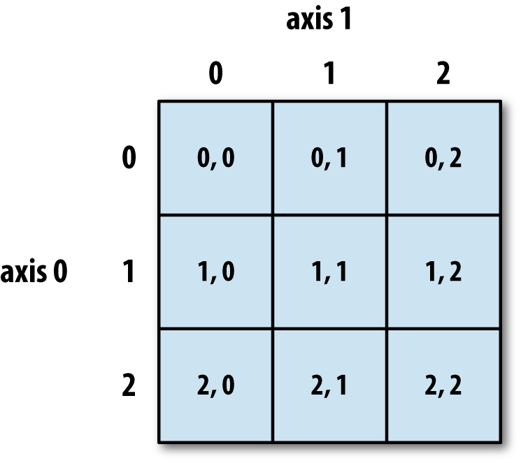
More generally (e.g. for arrays with additional dimensions), the last index in the sequence is the one which is stepped through the fastest in memory, i.e. we read along the columns before we get to the next row.
The size method gives the total number of elements in the array. We can also output the data type using the dtype method:
print("Array c:")
print("total number of elements: ",c.size)
print("data type of elements: ", c.dtype)
Array c:
total number of elements:  24
data type of elements:  int64
Array elements can consist of all the different data types. Unless otherwise specified, the type will be chosen that best fits the values you use to create the array.
Just like lists, arrays can be iterated through using loops, starting with the first axis:
print("For array a:")
for val in a:
    print(val,val**(1/3))

print("For array c:")
for j, arr in enumerate(c):
    print("Sub-array",j,"=",arr)
    for k, vec in enumerate(arr):
        print("Vector",k,"of sub-array",j,"=",vec)
For array a:
1 1.0
2 1.2599210498948732
3 1.4422495703074083
For array c:
Sub-array 0 = [[ 1  2  3]
 [ 4  5  6]
 [ 7  8  9]
 [10 11 12]]
Vector 0 of sub-array 0 = [1 2 3]
Vector 1 of sub-array 0 = [4 5 6]
Vector 2 of sub-array 0 = [7 8 9]
Vector 3 of sub-array 0 = [10 11 12]
Sub-array 1 = [[21 22 23]
 [24 25 26]
 [27 28 29]
 [30 31 32]]
Vector 0 of sub-array 1 = [21 22 23]
Vector 1 of sub-array 1 = [24 25 26]
Vector 2 of sub-array 1 = [27 28 29]
Vector 3 of sub-array 1 = [30 31 32]
However, numpy allows much faster access to the component parts of an array through slicing, and much faster operations on arrays using the numpy ufuncs.
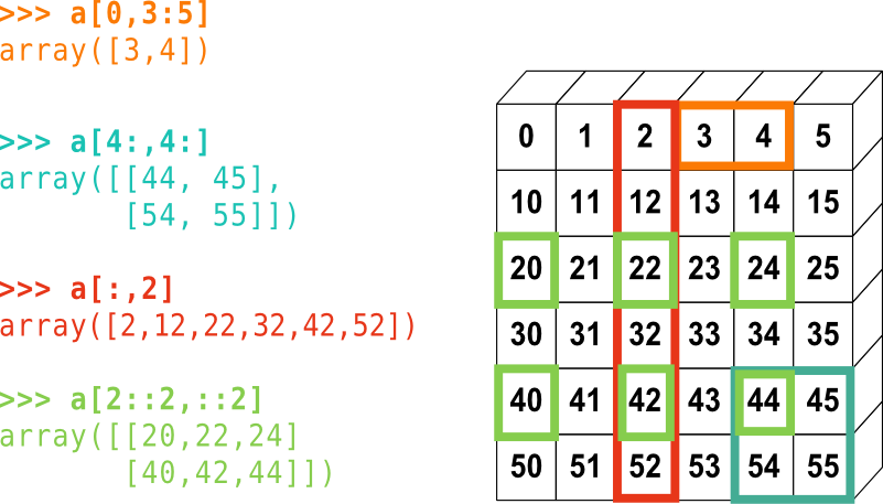
Array Slicing
Numpy arrays use the same rules for slicing as other Python iterables such as lists and strings.
Challenge
Without running the code first, what will the following print statements show?
d = np.array([0,1,2,3,4,5,6])

print(d[1:])
print(d[2:4])
print(d[-1])
print(d[::2])
print(d[-1:1:-1])
Solution
[1 2 3 4 5 6]
[2 3]
6
[0 2 4 6]
[6 5 4 3 2]
Slicing in two dimensions:
Challenge
Without running the code first, for the 3D matrix
cdefined earlier, what wouldprint(c[-1,1:3,::2])show?Solution
[[24 26]
[27 29]]
Making Simple Starting Arrays
It’s often useful to create a simple starting array of elements that can be modified or written to later on. Some simple ways to do this are shown here - the shape of the new array is specified using a tuple (or single integer if 1-D).
a = np.zeros((2,3)) # Fill the array with 0.
print("a =",a)

b = np.ones((4,4)) # Fill with 1.
print("b =",b)

c = np.full(10,3.0) # Fill with the value given
print("c =",c)
a = [[0. 0. 0.]
 [0. 0. 0.]]
b = [[1. 1. 1. 1.]
 [1. 1. 1. 1.]
 [1. 1. 1. 1.]
 [1. 1. 1. 1.]]
c = [3. 3. 3. 3. 3. 3. 3. 3. 3. 3.]
Making Evenly Spaced and Meshgrid Arrays
Besides building an array by hand, we can generate arrays automatically in a variety of ways.
Firstly, there are a variety of numpy functions to generate arrays of evenly spaced numbers.
arange generates numbers with a fixed interval (or step) between them:
a = np.arange(8) # Generates linearly spaced numbers. Default step size = 1.0 and start = 0.0
print("a =",a)

b = np.arange(start=3, stop=12, step=0.8) # The stop value is excluded
print("b =",b)
a = [0 1 2 3 4 5 6 7]
b = [ 3.   3.8  4.6  5.4  6.2  7.   7.8  8.6  9.4 10.2 11.  11.8]
The linspace function produces num numbers over a fixed range inclusive of the start and stop
value. geomspace and logspace work in a similar way to produce geometrically spaced values
(i.e. equivalent to linear spacing of the logarithm of the values). Note that we don’t need to specify
the argument names if they are written in the correct order for the function. There are also a number
of hidden default variables that may be specified if we wish - you should always check the
documentation for a function before you use it, either via an online search or using the help
functionality in the Notebook or python command-line.
c = np.geomspace(10.0,1e6,6)
print("c =",c)

d = np.logspace(1,6,6)
print("d =",d)
c = [1.e+01 1.e+02 1.e+03 1.e+04 1.e+05 1.e+06]
d = [1.e+01 1.e+02 1.e+03 1.e+04 1.e+05 1.e+06]
linspace and geomspace also accept arrays of stop, start and num to produce multidimensional arrays of numbers.
meshgrid is a particularly useful function that accepts N 1-D arrays to produce N N-D grids of coordinates. Each point in a grid shows the coordinate value of the corresponding axis. These can be used to, e.g. evaluate functions across a grid of parameter values or make 3-D plots or contour plots of surfaces.
x = np.linspace(21,30,10)
y = np.linspace(100,800,8)

xgrid1, ygrid1 = np.meshgrid(x,y,indexing='xy') # Use Cartesian (column-major order) indexing
xgrid2, ygrid2 = np.meshgrid(x,y,indexing='ij') # Use matrix (row-major order) indexing

print("Using Cartesian (column-major order) indexing:")
print("Grid of x-values:")
print(xgrid1,"\n") # Add a newline after printing the grid
print("Grid of y-values:")
print(ygrid1,"\n")

print("Using matrix (row-major order) indexing:")
print("Grid of x-values:")
print(xgrid2,"\n")
print("Grid of y-values:")
print(ygrid2,"\n")
Note that the printed grids begin in the top-left corner with the [0,0] position, but the column and row values are then reversed for xy vs ij indexing.
Using Cartesian (column-major order) indexing:
Grid of x-values:
[[21. 22. 23. 24. 25. 26. 27. 28. 29. 30.]
 [21. 22. 23. 24. 25. 26. 27. 28. 29. 30.]
 [21. 22. 23. 24. 25. 26. 27. 28. 29. 30.]
 [21. 22. 23. 24. 25. 26. 27. 28. 29. 30.]
 [21. 22. 23. 24. 25. 26. 27. 28. 29. 30.]
 [21. 22. 23. 24. 25. 26. 27. 28. 29. 30.]
 [21. 22. 23. 24. 25. 26. 27. 28. 29. 30.]
 [21. 22. 23. 24. 25. 26. 27. 28. 29. 30.]]

Grid of y-values:
[[100. 100. 100. 100. 100. 100. 100. 100. 100. 100.]
 [200. 200. 200. 200. 200. 200. 200. 200. 200. 200.]
 [300. 300. 300. 300. 300. 300. 300. 300. 300. 300.]
 [400. 400. 400. 400. 400. 400. 400. 400. 400. 400.]
 [500. 500. 500. 500. 500. 500. 500. 500. 500. 500.]
 [600. 600. 600. 600. 600. 600. 600. 600. 600. 600.]
 [700. 700. 700. 700. 700. 700. 700. 700. 700. 700.]
 [800. 800. 800. 800. 800. 800. 800. 800. 800. 800.]]

Using matrix (row-major order) indexing:
Grid of x-values:
[[21. 21. 21. 21. 21. 21. 21. 21.]
 [22. 22. 22. 22. 22. 22. 22. 22.]
 [23. 23. 23. 23. 23. 23. 23. 23.]
 [24. 24. 24. 24. 24. 24. 24. 24.]
 [25. 25. 25. 25. 25. 25. 25. 25.]
 [26. 26. 26. 26. 26. 26. 26. 26.]
 [27. 27. 27. 27. 27. 27. 27. 27.]
 [28. 28. 28. 28. 28. 28. 28. 28.]
 [29. 29. 29. 29. 29. 29. 29. 29.]
 [30. 30. 30. 30. 30. 30. 30. 30.]]

Grid of y-values:
[[100. 200. 300. 400. 500. 600. 700. 800.]
 [100. 200. 300. 400. 500. 600. 700. 800.]
 [100. 200. 300. 400. 500. 600. 700. 800.]
 [100. 200. 300. 400. 500. 600. 700. 800.]
 [100. 200. 300. 400. 500. 600. 700. 800.]
 [100. 200. 300. 400. 500. 600. 700. 800.]
 [100. 200. 300. 400. 500. 600. 700. 800.]
 [100. 200. 300. 400. 500. 600. 700. 800.]
 [100. 200. 300. 400. 500. 600. 700. 800.]
 [100. 200. 300. 400. 500. 600. 700. 800.]]
Editing and Appending
To edit specific values of an array, you can simply replace the values using slicing, e.g.:
z = np.zeros((8,6))
z[2::2,2:-1] = 1
print(z)
[[0. 0. 0. 0. 0. 0.]
[0. 0. 0. 0. 0. 0.]
[0. 0. 1. 1. 1. 0.]
[0. 0. 0. 0. 0. 0.]
[0. 0. 1. 1. 1. 0.]
[0. 0. 0. 0. 0. 0.]
[0. 0. 1. 1. 1. 0.]
[0. 0. 0. 0. 0. 0.]]
Additional elements can be added to the end of the array using append, or inserted before a specified index/indices using insert. Elements may be removed using delete.
a = np.arange(2,8)
print(a)
b = np.append(a,[8,9]) # Appends [8,9] to end of array
print(b)
c = np.insert(b,5,[21,22,23]) # Inserts [21,22,23] before element with index 5
print(c)
d = np.delete(c,[0,3,6]) # Deletes elements with index 0, 3, 6
print(d)
[2 3 4 5 6 7]
[2 3 4 5 6 7 8 9]
[ 2  3  4  5  6 21 22 23  7  8  9]
[ 3  4  6 21 23  7  8  9]
If we want to append to a multi-dimensional array, but do not specify an axis, the arrays will
be flattened (see ravel below) before appending, to produce a 1-D array. If we specify an axis, the array we append must have the same number of dimensions and the same shape along the other axes. E.g.:
a = np.zeros((3,8))
print(a,"\n")

b = np.append(a,np.ones((3,1)),axis=1)
print(b,"\n")

c = np.append(b,np.full((2,9),2.),axis=0)
print(c,"\n")

d = np.append(c,np.full((3,1),3.),axis=1)
print(d)
[[0. 0. 0. 0. 0. 0. 0. 0.]
 [0. 0. 0. 0. 0. 0. 0. 0.]
 [0. 0. 0. 0. 0. 0. 0. 0.]]

[[0. 0. 0. 0. 0. 0. 0. 0. 1.]
 [0. 0. 0. 0. 0. 0. 0. 0. 1.]
 [0. 0. 0. 0. 0. 0. 0. 0. 1.]]

[[0. 0. 0. 0. 0. 0. 0. 0. 1.]
 [0. 0. 0. 0. 0. 0. 0. 0. 1.]
 [0. 0. 0. 0. 0. 0. 0. 0. 1.]
 [2. 2. 2. 2. 2. 2. 2. 2. 2.]
 [2. 2. 2. 2. 2. 2. 2. 2. 2.]]

---------------------------------------------------------------------------
ValueError                                Traceback (most recent call last)
<ipython-input-65-6a09bd69590d> in <module>
      8 print(c,"\n")
      9
---> 10 d = np.append(c,np.full((3,1),3.),axis=1)
     11 print(d)

<__array_function__ internals> in append(*args, **kwargs)

~/anaconda3/lib/python3.7/site-packages/numpy/lib/function_base.py in append(arr, values, axis)
   4698         values = ravel(values)
   4699         axis = arr.ndim-1
-> 4700     return concatenate((arr, values), axis=axis)
   4701
   4702

<__array_function__ internals> in concatenate(*args, **kwargs)

ValueError: all the input array dimensions for the concatenation axis must match exactly, but along dimension 0, the array at index 0 has size 5 and the array at index 1 has size 3
Copying Arrays
You might think that we can make a direct copy
bof a Numpy arrayausinga = b. But look what happens if we change a value ina:a = [5.,4.,3.,9.] b = a print("b =",b) a[2] = 100. print("b =",b)b = [5. 4. 3. 9.] b = [ 5. 4. 100. 9.]The new array variable b is just another label for the array
a, so any changes toaare also mirrored inb, usually with undesirable results! If we want to make an independent copy of an array, we can use numpy’scopyfunction. Alternatively, we can carry out an operation on the original array which doesn’t change it (most operations write a new array by default). For example, both this:a = np.array([5.,4.,3.,9.]) b = np.copy(a) print("b =",b) a[2] = 100. print("b =",b)and this:
a = np.array([5.,4.,3.,9.])
b = a + 0
print("b =",b)
a[2] = 100.
print("b =",b)
will make
ba completely new array which starts out identical toabut is independent of any changes toa:b = [5. 4. 3. 9.] b = [5. 4. 3. 9.]
Reshaping and Stacking
Sometimes it can be useful to change the shape of an array. For example, this can make some data analysis easier (e.g. to make distinct rows or columns in the data) or allow you to apply certain functions which may otherwise be impossible due to the array not having the correct shape (e.g. see broadcasting in the next episode).
Numpy’s reshape function allows an array to be reshaped to a different array of the same size
(so the product of row and column lengths should be the same as in the original array). The
reshaping is done by reading out the elements in (C-like) row-major order (order='C'), i.e. last
index changing fastest, then the 2nd-to-last etc. or (Fortran-like) column-major order (order='F'),
with first index changing fastest. The elements of the new array are then populated on the same basis. For example:
a = np.linspace([1,11,21],[8,18,28],8)
print(a,"\n")

b = np.reshape(a,(2,12)) # The default order='C'
print(b,"\n")

c = np.reshape(a,(3,8))
print(c,"\n")

d = np.reshape(a,(3,8),order='F')
print(d)
[[ 1. 11. 21.]
 [ 2. 12. 22.]
 [ 3. 13. 23.]
 [ 4. 14. 24.]
 [ 5. 15. 25.]
 [ 6. 16. 26.]
 [ 7. 17. 27.]
 [ 8. 18. 28.]]

[[ 1. 11. 21.  2. 12. 22.  3. 13. 23.  4. 14. 24.]
 [ 5. 15. 25.  6. 16. 26.  7. 17. 27.  8. 18. 28.]]

[[ 1. 11. 21.  2. 12. 22.  3. 13.]
 [23.  4. 14. 24.  5. 15. 25.  6.]
 [16. 26.  7. 17. 27.  8. 18. 28.]]

[[ 1.  4.  7. 12. 15. 18. 23. 26.]
 [ 2.  5.  8. 13. 16. 21. 24. 27.]
 [ 3.  6. 11. 14. 17. 22. 25. 28.]]
It’s common to want to reshape the array so that the columns are swapped into rows and vice
versa, i.e. the equivalent of a matrix transpose.
This cannot be done using reshape since the function reads along whole rows
(or columns) as it populates the new array. Instead, you can use the transpose function
or the .T method:
e = np.transpose(a)
print(e,"\n")

f = a.T
print(f,"\n")
[[ 1.  2.  3.  4.  5.  6.  7.  8.]
 [11. 12. 13. 14. 15. 16. 17. 18.]
 [21. 22. 23. 24. 25. 26. 27. 28.]]

[[ 1.  2.  3.  4.  5.  6.  7.  8.]
 [11. 12. 13. 14. 15. 16. 17. 18.]
 [21. 22. 23. 24. 25. 26. 27. 28.]]
It’s sometimes useful to flatten a multi-dimensional array, i.e. read it out into a single dimension.
This is often also done by functions where the inputs are multi-dimensional and the output is otherwise not defined or ambiguous (e.g. if an axis to operate on is not specified). Flattening can be done using the ravel function. As for reshape, an order argument can be given to tell the function which index to read first.
g = np.ravel(a)
print(g,"\n")

h = np.ravel(a,order='F')
print(h)
[ 1. 11. 21.  2. 12. 22.  3. 13. 23.  4. 14. 24.  5. 15. 25.  6. 16. 26.
  7. 17. 27.  8. 18. 28.]

[ 1.  2.  3.  4.  5.  6.  7.  8. 11. 12. 13. 14. 15. 16. 17. 18. 21. 22.
 23. 24. 25. 26. 27. 28.]
Finally, there are a number of useful functions for “stacking” arrays together, which is useful when combining e.g. arrays of different variables obtained from the same series of measurements. For example, column_stack can be used to stack together 1-D arrays as columns or 2-D arrays on top of one another. hstack and vstack stack arrays in sequence horizontally (i.e. by column) or vertically (by row):
arr1 = np.arange(8)
arr2 = np.arange(11,19)
print(arr1,arr2,"\n")

print(np.column_stack((arr1,arr2)),"\n")

print(np.hstack((arr1,arr2)),"\n")

print(np.vstack((arr1,arr2)))
[0 1 2 3 4 5 6 7] [11 12 13 14 15 16 17 18]

[[ 0 11]
 [ 1 12]
 [ 2 13]
 [ 3 14]
 [ 4 15]
 [ 5 16]
 [ 6 17]
 [ 7 18]]

[[ 0  1  2  3  4  5  6  7]
 [11 12 13 14 15 16 17 18]]

[ 0  1  2  3  4  5  6  7 11 12 13 14 15 16 17 18]

[[ 0  1  2  3  4  5  6  7]
 [11 12 13 14 15 16 17 18]]
These functions can be used to stack arrays with multiple dimensions, with the requirement that they have the same shape for all axes except the axis along which they are being stacked.
stack is a more generic stacking function which is useful for stacking arrays of arbitrary dimension
along a new axis. Analogous functions, split, vsplit and hsplit exist to split an array into
multiple sub-arrays along various axes.
Reading Data from Files into Arrays
Numpy has a powerful function for reading data from text files: genfromtxt. It can automatically
skip commented text such as headers or (if the number of lines to be skipped is given),
read in variable names from the line preceding the data.
The function can split data around specified delimiters, work out data formats automatically and
the user can choose which columns of data to read in to an array.
Variable names and/or formats can also be specified as function arguments.
To see how to use it, we’ll first create a file:
var1 = np.geomspace(100.0,1000.0,5)
var2 = np.linspace(1.0,2.0,5)
var3 = np.arange(5)

with open('test_file1.txt', 'w') as f:
    f.write('# This is a header line\n')
    f.write('# This is another header line, the variables are next\n')
    f.write('# var1 var2 var3\n')
    for i, value in enumerate(var1):
        f.write(str(value)+' '+str(var2[i])+' '+str(var3[i])+'\n') # Remember you can only write a single string
Now we will read the data back in using genfromtxt:
data = np.genfromtxt('test_file1.txt', comments='#') # Will skip lines beginning with 'w'
print(data)
[[ 100.            1.            0.        ]
[ 177.827941      1.25          1.        ]
[ 316.22776602    1.5           2.        ]
[ 562.34132519    1.75          3.        ]
[1000.            2.            4.        ]]
In this case, the data on the file has been read in as an array, with each row in the file corresponding to a row in the array. Note also
that genfromtxt assumes as a default that the data values are of data-type float.
Now let’s look at reading in more complex data consisting of strings and numbers:
var1 = ['a','b','c','d','e']
var2 = np.linspace(1.0,2.0,5)
var3 = np.arange(5)

with open('test_file2.txt', 'w') as f:
    f.write('# This is a header line\n')
    f.write('# This is another header line, the variables are next\n')
    f.write('# var1 var2 var3\n')
    for i, value in enumerate(var1):
        f.write(value+' '+str(var2[i])+' '+str(var3[i])+'\n')
If we use genfromtxt with argument dtype=None, the function will guess the correct data types based on the input values.
data = np.genfromtxt('test_file2.txt', comments='#', dtype=None)
print("Data array:",data,"\n")
print("Data dtype:",data.dtype)
Data array: [(b'a', 1.  , 0) (b'b', 1.25, 1) (b'c', 1.5 , 2) (b'd', 1.75, 3)
 (b'e', 2.  , 4)]

Data dtype: [('f0', 'S1'), ('f1', '<f8'), ('f2', '<i8')]
This format is not a standard numpy array but a structured array. In the printed version of the array, each component in brackets represents a
row of the data. If we look at the dtype it shows us a tuple for each column which gives the field name and dtype for each column. Field
names (quoted as a string in square brackets, but not as an index) can be used to reference a given column of the data:
col2 = data['f1']
print(col2)

print(data['f0'][1]) # This returns the 2nd value from the first column (field f0)
[1.   1.25 1.5  1.75 2.  ]
b'b'
So far, so good. But the b prefix to the strings from the first column have been read in as bytes literals - that is, the letters are assumed to
represent a value in bytes and cannot be used as str values would (e.g. concatenated with other strings), without converting them first.
We can also tell genfromtxt which format each of the data columns should be in:
data = np.genfromtxt('test_file2.txt', comments='#', skip_header=2, names=True, dtype=('U10','f8','i4'))
print("Data array:",data,"\n")
print("Data dtype:",data.dtype)
Data array: [('a', 1.  , 0) ('b', 1.25, 1) ('c', 1.5 , 2) ('d', 1.75, 3)
 ('e', 2.  , 4)]

Data dtype: [('var1', '<U10'), ('var2', '<f8'), ('var3', '<i4')]
Where U10, f8 and i4 refer to respectively to a unicode string of up to 10 characters, 64-bit (8 byte) float and 32-bit (4 byte) integer. In this example, we also told genfromtxt to read the column names (names=True) which it looks for in the line after any skipped
header lines (hence we tell it how many lines to skip, using skip_header=2). We can also specify the names of the columns using the names
argument (e.g. names=['mystring','myfloat','myint'] or in the dtype argument using a sequence of tuples:
dtype=[('mystring','<U10'),...].
genfromtxt has many other arguments which may be useful, as usual it is good to read the online documentation for this important function.
Finally, it’s worth noting that python has useful functions to write arrays to files, including savetxt to save to a text file, as well as save (and variants of it), which can write to a special binary numpy file format which allows more compressed file storage and faster input of saved
arrays to a program.
Selecting Data: Conditional Operations on Arrays
A very powerful feature of numpy arrays is that items can be very easily selected from the arrays via conditional statements that operate on the contents of the array. In this way, it is possible to select not only the contents of a particular array, but also matched values in corresponding arrays of other variables, where the array elements correspond one-to-one to those in the array used to make the selection.
For example, consider a light curve from a periodic variable star, which we simulate and plot below:
time = np.arange(200) # time in days
flux = 1.0 + 0.4*np.sin(2*np.pi*time/23.0 + np.pi/3) # generate period 'light curve' with period 23 days
error = np.random.uniform(0.1,0.3,size=len(time)) # randomly generate error bar size from uniform distribution
flux = flux + error*np.random.normal(size=len(time)) # Now add normally distributed statistical error to flux


import matplotlib.pyplot as plt
# Plot in the notebook:
%matplotlib inline

plt.figure()
# Plot datapoints with error bars - ls=' ': switch off line through the data points:
plt.errorbar(time,flux,yerr=error,ls=' ',marker='o',ms=4)
plt.xlabel('Time (days)',fontsize=12)
plt.ylabel('Flux (arbitrary units)',fontsize=12)
plt.show()
This should plot something like this (your simulation will use different random numbers so will be similar but not identical):
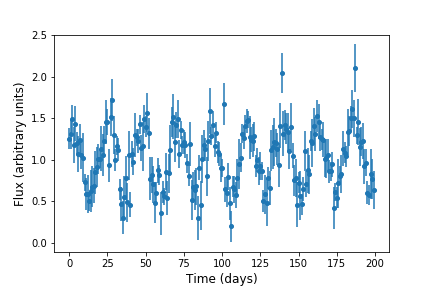
Now imagine that for some reason (e.g. a problem with the instrument on the telescope, or poor weather) we don’t trust the
data between days 75 and 95. We can use a conditional statement to create new arrays which only contain the elements
corresponding to time < 75 or time > 95):
time2 = time[(time < 75) | (time > 95)]
flux2 = flux[(time < 75) | (time > 95)]
error2 = error[(time < 75) | (time > 95)]

plt.figure()
plt.errorbar(time2,flux2,yerr=error2,ls=' ',marker='o',ms=4)
plt.xlabel('Time (days)',fontsize=12)
plt.ylabel('Flux (arbitrary units)',fontsize=12)
plt.show()
Which looks like this, i.e. with the data points removed:
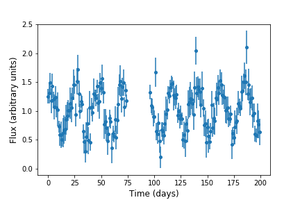
It’s good to bear in mind how such conditional selection on numpy arrays works. Firstly, the selection condition creates a Boolean array of
equal shape
as the original array(s) used to select, but filled with the truth values, True and False according to whether the condition is satisfied or not.
Now, remember that square brackets after an array name are used to select indices from the array. By putting the Boolean array inside the
square brackets (or the condition which generates it), we automatically select only from the True values. This method is called Boolean
masking. It is important that the shape of the Boolean array matches that of the array to be selected from (which should therefore also match the shape of the array(s) used to create the Boolean array).
Challenge
Finally, you can practice some of what you have learned about reading in and selecting from arrays, using the
KNMI_20200825.txtdata file of data from Dutch meteorological stations.First, use
genfromtxtto read in the data and automatically assign variable names and data types (note that there are 97 lines in the header before the line containing the variable names). Then, write a function which can take the data array, a station number and a temperature in Celsius and return the percentage of days recorded from that station with maximum temperature exceeding that value. Use your function to calculate the percentage of recorded days exceeding 30 degrees Celsius at the stations in Ijmuiden (station # 225) and Eindhoven (station # 370). Remember that the data records temperature in units of 0.1 C!Note: to be consistent with possible missing data for variables which
genfromtxtassigns as integer, float or string types, thegenfromtxtwill probably assign the value -1 to the data which are missing. This is problematic, because these values might be mistaken for actual values of the variables. It’s a good idea to change this using thegenfromtxtargumentfilling-values, e.g. set that argument to be-9999, which won’t be confused with any actual variable values. When you calculate with the data, be sure to remove these values from the array before calculating, e.g. you can filter using the condition that the value!= -9999.Solution
First read in the data:
data = np.genfromtxt('KNMI_20200825.txt',delimiter=',',comments='#',skip_header=97,names=True,dtype=None,filling_values=-9999)Now define the function:
def frac_max_temp(data,stn_num,max_limit_cels):
    """Function to calculate percentage of recorded days for a given station with maximum temp TX
    above a given temperature value.

    Inputs are:
    data: the structured KNMI data array
    stn_num: station number
    max_limit_cels maximum temperature lower limit in Celsius

    Output: print the percentage of recorded days exceeding the maximum temp. given"""

    data_stn = data[data['STN'] == stn_num] # Select data for that station only
    data_stn = data_stn[data_stn['TX'] != -9999]  # Ignore days without recorded max. temp

    # Now calculate the percentage from the decimal fraction of recorded days exceeding the given temp
    # remember to multiply limit by a factor 10 since data records temp as number of 0.1 Celsius increments
    pc_days = 100 * len(data_stn[data_stn['TX'] > 10*max_limit_cels]) / len(data_stn)

    # And print the result, rounded to 2 decimal places
    print("For station",stn_num,",",round(pc_days,2),"per cent of recorded days show max. temperature above",
          max_limit_cels," celsius.")

    return
and run the function for Ijmuiden and Eindhoven for days above 30 degrees C.
frac_max_temp(data,225,30.) # Ijmuiden
frac_max_temp(data,370,30.) # Eindhoven
For station 225 , 0.29 per cent of recorded days show max. temperature above 30.0 celsius. For station 370 , 1.41 per cent of recorded days show max. temperature above 30.0 celsius.
Key Points
Numpy arrays can be created from lists using
numpy.arrayor via other numpy functions.Like lists, numpy arrays are indexed in row-major order, with the last index read out fastest.
Numpy arrays can be edited and selected from using indexing and slicing, or have elements appended, inserted or deleted using using
numpy.append,numpy.insertornumpy.delete.Numpy arrays must be copied using
numpy.copyor by operating on the array so that it isn’t changed, not using=which simply assigns another label to the same array, as for lists.Use
numpy.reshape,numpy.transpose(or.T) to reshape arrays, andnumpy.ravelto flatten them to a single dimension. Variousnumpystackfunctions can be used to combine arrays.
numpy.genfromtxtcan read data into structured numpy arrays. Columns must be referred to using the field name given to that column when the data is read in.Conditional statements can be used to select elements from arrays with the same shape, e.g. that correspond to the same data set.
Array Calculations with Numpy
Overview
Teaching: 20 min
Exercises: 30 minQuestions
How can I perform calculations on large arrays quickly, using numpy functions?
Objectives
Use the library of numpy functions for fast array calculations.
Understand how arrays of different shapes can be operated on using broadcasting.
Mask arrays to hide unwanted data and use masked array ufuncs to operate on them.
Write functions to perform complex operations on arrays.
Numpy offers an enormous range of pre-compiled functions in its numerical libraries, which allow a wide range of tasks to be completed on large arrays of data with speeds comparable to or approaching those of dedicated compiler languages such as Fortran or C++. We describe some examples of some of these functions here, but you should read the Numpy documentation online to find many more. A good general rule is that if you can think of a numerical method or function that you want to use, it is already implemented in numpy (or possibly scipy). So googling what you want to do together with the terms numpy or scipy is a good way to find what you need.
More on Numpy Ufuncs
Numpy ufuncs are pre-compiled (usually in C) functions that that operate on ndarray type objects (i.e. numpy arrays). They operate element-wise (item by item) on the array and support type casting (python will try to make non matching data types work) and broadcasting (i.e. python will try to make different array shapes work, see below). Most mathematical functions are available (we include some examples in this Episode and elsewhere in this lesson) and it’s also possible to write your own.
Ufuncs which operate on arrays come in two main flavours: unary ufuncs operate on a single array, while binary ufuncs operate on a pair of arrays. An example of binary ufuncs are the standard mathematical operators, which are wrappers for the underlying numpy functions:
import numpy as np

a = np.linspace(10,50,5)
b = np.arange(5)
print("a =",a)
print("b =",b,"\n")

print("a + b =",a+b,"is the same as np.add(a,b) =",np.add(a,b))
print("a - b =",a-b,"is the same as np.subtract(a,b) =",np.subtract(a,b))
print("-a =",-a,"is the same as np.negative(a) =",np.negative(a))
print("a * b =",a*b,"is the same as np.multiply(a,b)=",np.multiply(a,b))
print("a / b =",a/b,"is the same as np.divide(a,b)=",np.divide(a,b))
print("a // b =",a//b,"is the same as np.floor_divide(a,b)=",np.floor_divide(a,b))
print("a**b =",a**b,"is the same as np.power(a,b)=",np.power(a,b))
print("a % b =",a%b,"is the same as np.mod(a,b)=",np.mod(a,b))
a = [10. 20. 30. 40. 50.]
b = [0 1 2 3 4]

a + b = [10. 21. 32. 43. 54.] is the same as np.add(a,b) = [10. 21. 32. 43. 54.]
a - b = [10. 19. 28. 37. 46.] is the same as np.subtract(a,b) = [10. 19. 28. 37. 46.]
-a = [-10. -20. -30. -40. -50.] is the same as np.negative(a) = [-10. -20. -30. -40. -50.]
a * b = [  0.  20.  60. 120. 200.] is the same as np.multiply(a,b)= [  0.  20.  60. 120. 200.]
a / b = [        inf 20.         15.         13.33333333 12.5       ] is the same as np.divide(a,b)= [        inf 20.         15.         13.33333333 12.5       ]
a // b = [nan 20. 15. 13. 12.] is the same as np.floor_divide(a,b)= [nan 20. 15. 13. 12.]
a**b = [1.00e+00 2.00e+01 9.00e+02 6.40e+04 6.25e+06] is the same as np.power(a,b)= [1.00e+00 2.00e+01 9.00e+02 6.40e+04 6.25e+06]
a % b = [nan  0.  0.  1.  2.] is the same as np.mod(a,b)= [nan  0.  0.  1.  2.]
Writing these operations using the common mathematical operators is quicker than using the full numpy function names - and they follow the usual mathematical rules for order of operation, with powers calculated first, then division and multiplication then addition and subtraction. But you should remember that these are array operations and not operations on single variables!
Broadcasting
Binary ufuncs operate on two arrays (e.g. addition or multiplication of two arrays, to give a simple example). If the arrays have the same shape (same number of dimensions, each with the same size) the operation is applied to the corresponding pairs of elements in the array (i.e. the pair of elements with the same indices).
However, a great advantage of numpy’s arrays and ufuncs is that they allow broadcasting. Numpy’s broadcasting rules allow binary ufuncs to be applied to arrays of different shapes, provided that the shape of the smaller array can be mapped on to the same shape as the larger array in an unambiguous way. The broadcasting rules can be simplified to:
If both arrays have a different number of dimensions, the shape of the one with fewer dimensions is padded (on the left side of the shape tuple) with dimensions of size 1 so that the dimensions are now matched.
If the shapes are not the same in any dimension, the array with size 1 in that dimension is extended in size (repeating the same values), to match the other array.
However, if the sizes in a given dimension don’t match and neither is equal to 1 an error is raised.
The figure below (created using the code here) shows examples of successful broadcasting.
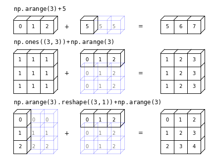
Challenge
Write a function that can take an input array of dates expressed with integer type as YYYYMMDD (e.g. 19950325, as read in by
genfromtxtfrom the KNMI data set) and returns three separate arrays of year, month and the day of the month. To calculate these quantities you should use only the numpy functions corresponding to standard mathematical operations with math symbol wrappers (see above).Hint
To get you started, this is how you can find the year:
year = date // 10**4Solution
def get_ymd(date):
    '''Takes as input the date as integer type YYYYMMDD and returns year, month
    (as integer 1-12) and day of the month'''

    year = date // 10**4
    month = date // 10**2 % 100
    day = date % 100

    return year, month, day
Common mathematical functions
Besides the common mathematical operators, there are ufuncs for all of the common mathematical functions. E.g.:
print("Square root of a:",np.sqrt(a))
print("Exponential of b:",np.exp(b))
print("log_10(a) =",np.log10(a)) # Log in base 10
print("ln(a) =",np.log(a)) # Natural log
print("log_2(a) =",np.log2(a)) # Log in base 2
print("\n\n")

angles = np.linspace(0.,2*np.pi,10) # Pi can be called with np.pi
print("Angles in radians:",angles)
print("Angles in degrees:",np.degrees(angles)) # To go from degrees to radians, use np.radians

print("tan(b): ",np.tan(a)) # Functions include inverse (arctan etc.) and other trig functions
Square root of a: [3.16227766 4.47213595 5.47722558 6.32455532 7.07106781]
Exponential of b: [ 1.          2.71828183  7.3890561  20.08553692 54.59815003]
log_10(a) = [1.         1.30103    1.47712125 1.60205999 1.69897   ]
ln(a) = [2.30258509 2.99573227 3.40119738 3.68887945 3.91202301]
log_2(a) = [3.32192809 4.32192809 4.9068906  5.32192809 5.64385619]


Angles in radians: [0.         0.6981317  1.3962634  2.0943951  2.7925268  3.4906585
 4.1887902  4.88692191 5.58505361 6.28318531]
Angles in degrees: [  0.  40.  80. 120. 160. 200. 240. 280. 320. 360.]
tan(b):  [ 0.64836083  2.23716094 -6.4053312  -1.11721493 -0.27190061]
Conditional functions
There are also a large number of useful numpy functions for manipulating and selecting from arrays. For example
numpy.whereallows the user to set a condition to be applied to each element of the array (given by the first argument), with two different results to be applied, according to whether the condition is satisfied or not (second and third argument respectively). For example, what function would the following code produce?t = np.linspace(0,10*np.pi,1000) a = np.sin(t) b = np.where(a > 0,1,0) plt.figure() plt.plot(t,b) plt.xlabel('t',fontsize=12) plt.ylabel('b',fontsize=12) plt.show()Solution
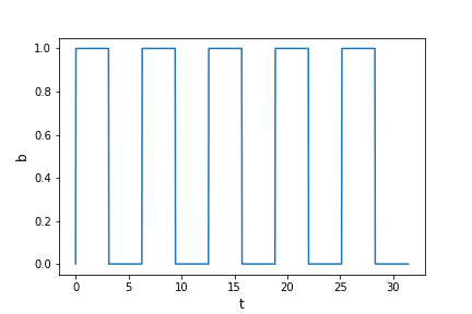
A square wave function!
In this case, constants were given as the results for the
TrueorFalsecases of the condition, but functions could also be specified instead.
Random numbers and statistics
Numpy’s numerical libraries include a large number of functions that are useful for statistical simulations (e.g. generating random numbers), as well as calculating standard statistical quantities. For example, random numbers can be generated for a large number of simulations using numpy.random and suffixing with the required distribution (and its arguments - see the numpy documentation for details). E.g.:
a = np.random.normal(size=10) # drawn from normal distribution (mean 0, standard deviation 1)
b = np.random.uniform(2,6,size=10) # drawn from uniform distribution with min. 2, max. 6

print("a = ",a,"\n")
print("b =",b)
The random numbers will change every time you generate them, so they won’t match the example
values shown below. To prevent this you could fix the random number generating ‘seed’ to the
same value each time (e.g. using numpy.random.seed). Fixing random number seeds is generally
a bad idea, as you almost always need your generated values to be statistically independent
each time.
a =  [-0.30022351 -0.2436521   0.82529598  1.45559054  2.81468678  0.63432945
  0.45292206 -0.7189043  -1.5688999  -2.07679378]

b = [4.91409402 5.20504639 4.10317644 4.52392586 4.12252377 5.19390016
 2.63697377 2.09074333 5.82355927 5.00880279]
There are a large number of functions to calculate statistical properties of data, e.g.:
mean = np.mean(a)
std_dev = np.std(a,ddof=1)
median = np.median(a)

# For the standard deviation of a sample, the degrees of freedom ddof=1
print("For a, mean =",np.mean(a),"median =",np.median(a),"and standard deviation =",np.std(a,ddof=1))
print("For b, mean =",np.mean(b),"median =",np.median(b),"and standard deviation =",np.std(b,ddof=1))

# The statistical quantities for a large random sample should be closer to the population ('true') values:
c = np.random.normal(size=100000)
d = np.random.uniform(2,6,size=100000)

print("For c, mean =",np.mean(c),"median =",np.median(c),"and standard deviation =",np.std(c,ddof=1))
print("For d, mean =",np.mean(d),"median =",np.median(d),"and standard deviation =",np.std(d,ddof=1))
For a, mean = 0.1274351220779665 median = 0.10463498050131667 and standard deviation = 1.4379104160216345
For b, mean = 4.36227458161702 median = 4.719009939469249 and standard deviation = 1.1807239934047047
For c, mean = -0.003106470300092659 median = -0.0020945245248079037 and standard deviation = 1.0019999302839593
For d, mean = 4.00191762092067 median = 4.001883767677743 and standard deviation = 1.1542783586377883
For multi-dimensional data sets the default is to flatten the array and calculate a single statistical quantity for all the values, but by specifying the axis as an integer or tuple of integers, quantities can be calculated along specific dimensions of the array. This can be useful if you want to arrange your data into many sub-samples corresponding to, e.g. columns in the array, and calculate separate statistical quantities for each sub-sample. For example:
x = np.linspace(1,6,10)
y = np.random.normal(x,np.sqrt(x),size=(20,10)) # Mean and standard deviation increase with x

y_mean = np.mean(y,axis=0) # Measure mean along each column of 20 values
y_std = np.std(y,axis=0,ddof=1) # Measure standard deviation

print("Means =",y_mean)
print("Standard deviations =",y_std)
Means = [1.10406239 1.79198285 2.41687801 2.61184147 2.37594309 3.46102472 4.72351714 4.66671086 4.68688962 6.8386863 ]
Standard deviations = [1.21478777 1.46095133 1.53221715 1.89578884 1.66559555 2.28753281 1.90451327 2.55568894 2.19337894 2.31425862]
Numpy functions like these can be used to handle data sets, but for more extensive analysis, especially with large and complex data sets Pandas (which is based in large part on numpy and scipy) is a more suitable and versatile library.
Masked Arrays
In some situations your array may contain elements with no data, bad data, or data which you wish to filter from your analysis for some other reason. You can remove this data using a condition to filter out the elements you don’t want, but this only works if the resulting array can be flattened and you don’t need to preserve its shape. However, if you want to keep the shape of your data array (e.g. for statistical calculations along a particular axis), it is useful to create a masked array. These can be created using the
numpy.mamodule, which also includes equivalents of common numpy functions that can be applied to masked arrays (for which the usualnumpyfunctions will not work).First, we will add some
nanvalues in random locations in theyarray we generated previously:# First randomly select indices of elements from y to change values to NaN in new array y2 cols = np.random.random_integers(0,9,size=20) rows = np.random.random_integers(0,19,size=20) y2 = np.copy(y) y2[rows,cols] = np.nan y2_mean = np.mean(y2,axis=0) # Measure mean along each column of 20 values y2_std = np.std(y2,axis=0,ddof=1) # Measure standard deviation print("Means =",y2_mean) print("Standard deviations =",y2_std)Means = [ nan nan nan nan nan 3.46102472 nan nan nan nan] Standard deviations = [ nan nan nan nan nan 2.28753281 nan nan nan nan]Any columns containing
nanwill result innanfor the statistics calculated along those columns. We can produce a masked array withnanvalues masked. One way to create a masked array is to use themasked_arrayfunction with a Boolean array ofTrue/Falsevalues with the same shape as the array to be masked, e.g.:y2_ma = np.ma.masked_array(y2,np.isnan(y2)) y2_ma_mean = np.ma.mean(y2_ma,axis=0) # Measure mean along each column of 20 values y2_ma_std = np.ma.std(y2_ma,axis=0,ddof=1) # Measure standard deviation print("Means =",y2_ma_mean) print("Standard deviations =",y2_ma_std)Means = [0.8922926559222217 1.679217577416684 2.432410192332734 2.5727061459634673 2.2115371803066557 3.4610247170590283 4.475816052299866 4.786879589526783 4.743040460933355 6.887791934103876] Standard deviations = [1.1636287759233295 1.5121734615501945 1.6169210355493306 1.974709637455112 1.5354844835950414 2.2875328102951253 1.8266358576564314 2.5670126872971335 2.236916568224871 2.3669453874421658]We must be careful with any statistical measures from masked data, in case the missing values cause the measurements to be biased in some way.
Using Numpy to calculate with the KNMI data
Now we can use the methods we have looked at above to quickly calculate monthly quantities from the KNMI meteorological data, and plot them. First, read in the data (substituting missing values with
-9999:data = np.genfromtxt('KNMI_20200825.txt',delimiter=',',comments='#',skip_header=97,names=True,dtype=None,filling_values=-9999)Challenge Part 1
For the first part of the challenge, write a function which takes as input the structured data array read in above, the station number and the name of the variable you want to plot (you can see the variable names using
print data.dtypeto show the field information for the structured array). The function should select only the dates and the variable values for that station and when the quantity corresponding to that variable was measured (see the solution to the Challenge at the end of the previous Episode).Next, the function should recalculate the dates as arrays of integer type for the day, month and year (see the Challenge earlier in this Episode), and assign the values of the variable to a 3-D array, where the axes of the array correspond to year (measured since the first year when data was taken), month and day of the month. Before assigning values to the array, create your array so that it is already filled with
nanvalues, to identify positions in the array that correspond to dates with no data for that variable, or which do not correspond to real dates (such as Feb 31).Finally, your function should output the resulting 3-D array as well as the integer value of the first year in the return data array, so that year values corresponding to that axis can be determined (the days and months should be self-evident from the indices).
If you find this part too difficult or time consuming, you can look at the solution and skip ahead to the next part. This first part is really focussed on array manipulation using the principles discussed in the previous Episode. The second part focusses on using methods discussed in this Episode.
Part 1 Solution
def get_3d_data(data,stn_num,varname):
    '''Read in structured data array, station number (int) and variable name (str),
    select data for that station and variable only, and then assign the data to a
    3D array where axes correspond to the year, month and day.
    Output: 3D data array and the starting year for the data'''

    # First select date and variable values for given station number
    data_stn = data[data['STN'] == stn_num] # Select data for that station only
    data_stn = data_stn[data_stn[varname] != -9999] # Only include data when the
    selected variable was measured
    year, month, day = get_dmy(data_stn['YYYYMMDD'])
    variable =  data_stn[varname]

    # Now lets define a 3D array for our variable, where each axis corresponds to a
    year, month and day.
    # First, set the dimensions:

    y_len = (year[-1]-year[0])+1  # This assumes years are in chronological order
    m_len = 12  # 12 months in a year...
    d_len = 31 # Allow up to 31, excess days are filled with NaN and we should filter
    them in calculations

    # Set up the 3D array:
    data_array = np.full((y_len,m_len,d_len),np.nan)

    # Now fill the 3D array with the corresponding data values.
    # indices start at 0 so days/months should be shifted back by 1
    data_array[year-year[0],month-1,day-1] = variable

    return data_array, year[0]
Challenge Part 2
Now write a function that does the following:
- Takes as input the original structured array produced by
genfromtxtfrom the KNMI data file, a station number and a list of variable names- Looping through the list of variable names, then within the loop:
- Create a 3-D data array using the function written in Part 1 of this Challenge.
- Create a masked version of the 3-D array to ignore the elements with
nan.- Use the masked array to calculate the mean values for the 12 months in the year (i.e. averaging the data over all years and days in that month)
- Plot the means vs. month, so that all the variables in the list are plotted in the same plot (use
plt.show()outside the loop at the end of the function). For extra brownie points, add a legend which shows the variable names vs. plot symbol/colour (depending on the type of plot) and correct by a factor 10 the variables that are given in tenths of a unit, to show them in the normal units.Use your function to plot the monthly average of the daily minimum (TN), mean (TG) and maximum (TX) temperatures for a selected station.
Hint
To plot a legend you can include an argument
labelin the plotting function call (e.g.plt.plot), where the value of label is a string, and then include the functionplt.legend()before plotting.Part 2 Solution
def plot_monthly_allyears(data,stn_num,var_list):
    '''Read in the structured data array of KNMI data, station number and list of variables.

    Loops through the list of variables to obtain a 3-D (year,month,day) array for that variable,
    masks the array to ignore missing data and calculate the means (over all years) for each month.
    Then plot the variable so all appear on the same plot.

    Does not return anything.'''

    months = ['Jan','Feb','Mar','Apr','May','Jun','Jul','Aug','Sep','Oct','Nov','Dec']
    plt.figure()
    for i, varname in enumerate(var_list):
        # Make 3D array for that variable
        data_array, year_start = get_3d_data(data,stn_num,varname)
        # Create a masked array to remove nan values
        data_array_ma = np.ma.masked_array(data_array,np.isnan(data_array))
        if (varname[0] in ('D','U','Q','V') or varname[-1] == 'H' or varname == 'SP'):
        # Find the mean value for each month by averaging over all years and days in that month
        means = np.ma.mean(data_array_ma,axis=(0,2))
        else:
        means = 0.1*np.ma.mean(data_array_ma,axis=(0,2))
        plt.plot(np.arange(1,13),means,label=varname,marker='o',linewidth=2,linestyle='-')
    # These plot commands apply to the whole plot so we can end the loop here
    plt.xticks(np.arange(1,13),months)
    plt.ylabel("Average Value",fontsize=12)
    plt.xlabel("Month",fontsize=12)
    plt.legend()
    plt.show()
    return
Now let’s plot the temperatures for Eindhoven:
plot_monthly_allyears(data,370,['TX','TG','TN'])
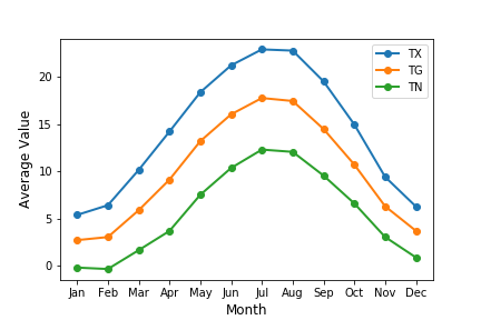
Key Points
Numpy ufuncs operate element-wise (item by item) on an array.
Common mathematical operators applied to numpy arrays act as wrappers for fast array calculations.
Binary ufuncs operate on two arrays: if the arrays have different shapes which are compatible, the operation uses broadcasting rules.
Many operations and numerical methods (such as random number generation) can be carried out with numpy functions.
Arrays can be masked to allow unwanted elements (e.g. with
nanvalues) to be ignored in array calculations using special masked array ufuncs.Define your own functions that carry out complex array operations by combining different numpy functions.
Numerical Methods with Scipy
Overview
Teaching: 40 min
Exercises: 0 minQuestions
What numerical methods are available in the Scipy library?
Objectives
Discover the wide range of numerical methods that are available in Scipy sub-packages
See how some of the subpackages can be used for interpolation, integration, model fitting and Fourier analysis of time-series.
Introducing Scipy
Scipy is a collection of packages and functions based on numpy, with a goal of performing scientific computation with numerical methods which have similar functionality as common numerical languages such as MATLAB, IDL and R. The scipy library is heavily integrated with numpy and matplotlib.
Scipy is organised into sub-packages covering different topics - you need to import them individually. The sub-packages are:
| Sub-package | Methods covered |
|---|---|
cluster |
Clustering algorithms |
constants |
Physical and mathematical constants |
fft |
Fast Fourier Transform routines |
integrate |
Integration and ordinary differential equation solvers |
interpolate |
Interpolation and smoothing splines |
io |
Input and Output |
linalg |
Linear algebra |
ndimage |
N-dimensional image processing |
odr |
Orthogonal distance regression |
optimize |
Optimization and root-finding routines |
signal |
Signal processing |
sparse |
Sparse matrices and associated routines |
spatial |
Spatial data structures and algorithms |
special |
Special functions |
stats |
Statistical distributions and functions |
mstats |
Statistical functions for masked arrays |
We’ll look at some examples here, but the sub-package topics will give you an idea of where to look for things online, by looking at their documentation. Also, as with numpy, you can usually find what you want by combining what you want to do with the names ‘scipy’, ‘numpy’ (or just ‘Python’) in a google search. The trick is figuring out the formal way to describe what it is that you are trying to do (although a verbal description of it will sometimes work!).
Check the function documentation!
It is very important that you always check the documentation for a scipy (or numpy) function before using it for the first time. This is not only to see what inputs the function requires (and what its outputs are), but also to check the assumptions that go into the function calculation (e.g. the
curve_fitfunction require errors on the data to be normally distributed). You should never use a function as a ‘black box’ without understanding the basics of what it is supposed to do and what special conditions are required for the results to make sense.For the functions described below, as you go through them take a look at the documentation (google the function name and ‘scipy’ but be sure to look at the latest version, or the one suitable for your installation of scipy). You will see that many functions have a lot of other capabilities, including a variety of additional arguments to control how they work, and sometimes additional methods that make them more versatile.
Interpolation
With the interpolation sub-package you can carry out 1-D interpolation using a variety of techniques (e.g. linear, cubic), taking as input 1-D arrays of \(x\) and \(y\) values and a set of new \(x\) values, for which the interpolated \(y\) values should be determined:
import numpy as np
import matplotlib.pyplot as plt
%matplotlib inline

from scipy.interpolate import interp1d

x = np.linspace(0, 10, num=11, endpoint=True)
y = np.cos(-x**2/9.0)
f = interp1d(x, y)
f2 = interp1d(x, y, kind='cubic')
f3 = interp1d(x, y, kind='nearest')

xnew = np.linspace(0, 10, num=100, endpoint=True)

plt.figure()
plt.plot(x, y, '-o')
plt.plot(xnew, f(xnew), '-')
plt.plot(xnew, f2(xnew), '--')
plt.plot(xnew, f3(xnew), ':')
plt.plot(x, y, '-o')
plt.xlabel('x',fontsize=14)
plt.ylabel('y',fontsize=14)
plt.tick_params(axis='both', labelsize=12)
plt.legend(['data','linear','cubic','nearest'], loc='best',fontsize=14)
plt.savefig('interpolation.png')
plt.show()
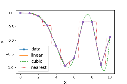
A variety of 1- and N-dimensional interpolation functions are also available.
Integration
Within scipy.integrate, the quad function is useful for evaluating the integral of a given
function, e.g. suppose we want to integrate any function \(f(x)\) within the boundaries \(a\) and
\(b\): \(\int_{a}^{b} f(x) dx\)
As a specific example let’s try \(\int_{0}^{\pi/2} sin(x) dx\), which we know must be exactly 1:
from scipy.integrate import quad

# quad integrates the function using adaptive Gaussian quadrature from the Fortran QUADPACK library

result, error = quad(np.sin, 0, np.pi/2)

print("Integral =",result)
print("Error =",error)
Besides the result, the function also estimates a numerical error (which arises due to the floating point accuracy, i.e. number of bits used for numbers, in the calculations).
Integral = 0.9999999999999999
Error = 1.1102230246251564e-14
Optimization and model-fitting
The scipy.optimize sub-package contains a large number of functions for optimization, i.e.
solving an equation to maximize or minimize (the more common situation) the result. These
methods are particularly useful for model-fitting, when we want to minimize the difference
between a set of model predictions and the data itself. To use these fully use these methods,
accounting for statistical errors, you should study statistical methods and data analysis,
which is beyond the scope of this course. For now, we introduce a few of these methods
as a primer with a few simple use cases.
First we’re going to generate a sine wave time series, adding scatter to the data points with random numbers drawn from a normal distribution:
from scipy import optimize

x_data = np.linspace(-5, 5, num=50)
y_data = 2.9 * np.sin(1.5 * x_data) + np.random.normal(size=50)

# We know that the data lies on a sine wave, but not the amplitudes or the period.

plt.plot(x_data,y_data,"o")
plt.figure()
plt.plot(x_data,y_data,"o")
plt.xlabel('x',fontsize=14)
plt.ylabel('y',fontsize=14)
plt.show()
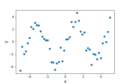
The scatter in the data means that the parameters of the sine-wave cannot be easily determined
from the data itself. A standard approach is to minimise the squared residuals (the residual is
the difference, data - model). Under certain conditions (if the errors are normally distributed),
this least squares minimization can be done using scipy.optimize’s curve_fit function.
First, we need to define the function we want to fit to the data:
# Set up a function with free parameters to fit to the data

def test_func(x, a, b):
    return a * np.sin(b * x)
Now we call curve_fit, giving as arguments our function name, the data \(x\) and \(y\)
values, and the starting parameters for the model (given as a list or array).
If no error bars on the data points are specified, curve_fit will return the best-fitting
model parameters which minimize the squared residuals, which we can also use to
plot the best-fitting model together with the data. We will not consider the case where
error bars are specified (which minimizes the so-called chi-squared statistic) or the
parameter covariance which is also produced as output (and which can be used to estimate
model parameter). These should be discussed in any course on statistical methods.
params, params_covariance = optimize.curve_fit(test_func, x_data, y_data, p0=[2, 2])
print("Best-fitting parameters = ",params)

plt.figure()
plt.plot(x_data,y_data,"o")
plt.plot(x_data,test_func(x_data,params[0],params[1]),"r")
plt.xlabel('x',fontsize=14)
plt.ylabel('y',fontsize=14)
plt.show()
Best fitting parameters: [2.70855704 1.49003739]
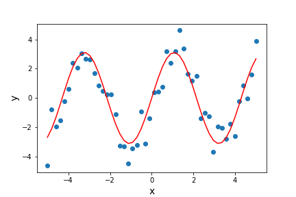
The best-fitting parameters are similar to but not exactly the same as the ones we used to generate the data. This isn’t surprising because the random errors in the data will lead to some uncertainty in the fitted parameter values, which can be estimated using a full statistical treatment of the fit results.
Besides model-fitting, we may want to simply find the minimum of a function (if the maximum is needed, it can usually be found by using minimization with the function to be maximized multiplied by -1!). For example, let’s find the minimum in this function:
def f(x):
    return x**2 + 10*np.sin(x)

x = np.arange(-10, 10, 0.1)

plt.figure()
plt.plot(x, f(x))
plt.xlabel('x',fontsize=14)
plt.ylabel('f(x)',fontsize=14)
plt.show()
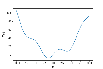
For general cases such as this (where we aren’t dealing with random errors that require
minimization of squared residuals), we can use methods provided by the scipy.optimize
function minimize. There are a wide range of optimization methods which minimize can use by changing the,
from ‘downhill simplex’ (such as Nelder-Mead) to conjugate gradient methods (e.g. BFGS).
You should look them up to find out how they work. They all have pros and cons.
result = optimize.minimize(f, x0=0, method='BFGS')

print("Results from the minimization are:",result)

plt.plot(x, f(x))
plt.plot(result.x, f(result.x),"ro",label="minimum")
plt.xlabel('x',fontsize=14)
plt.ylabel('f(x)',fontsize=14)
plt.legend(fontsize=14)
plt.show()
The result obtained by minimize is a compound object that contains all the information of the minimization attempt. result.fun gives the minimum value of the function and result.x
gives the best-fitting model parameters corresponding to the function minimum. The other
parameters depend on the method used, but may include the Jacobian (1st order
partial derivative of the function, evaluated at the minimum) and the Hessian (2nd order
partial derivative of the function, evaluated at the minimum) or its inverse (related to the
covariance matrix). The use of the 2nd-order derivatives should be considered in any
course covering statistical methods applied to data.
     fun: -7.945823375615215
hess_inv: array([[0.08589237]])
     jac: array([-1.1920929e-06])
 message: 'Optimization terminated successfully.'
    nfev: 18
     nit: 5
    njev: 6
  status: 0
 success: True
       x: array([-1.30644012])
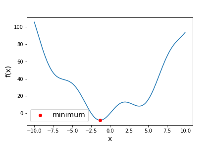
Fast Fourier Transforms
Fourier transforms can be used to decompose a complex time-series signal into its component frequencies of variation, which can yield powerful insights into the nature of the variability process, or important astrophysical parameters (such as the rotation period of a neutron star, or the orbital period of a planet or a binary system). Particularly useful are the class of Fast Fourier Transforms (FFT), which use clever numerical methods to reduce the number of operations needed to calculate a Fourier transform of a time-series of length \(n\), from \(n^{2}\) operations to only \(\sim n \ln(n)\).
Scipy’s fft sub-package contains a range of FFT functions for calculating 1-, 2- and N-D FFTs, as
well as inverse FFTs. Note that scipy.fft supercedes the former FFT subpackage scipy.fftpack. If you have an older version of Scipy, the code below will not work, but it should work if you change the name of the sub-package to fftpack (or even better, update your version of Scipy!).
First, let’s simulate a sinusoidal signal with a period of 0.5 s, embedded in Gaussian noise:
time_step = 0.02  # 0.02 s time bins
period = 0.5  # 0.5 s period

time = np.arange(0, 20, time_step)
sig = (np.sin(2 * np.pi / period * time) + 2.0 * np.random.randn(time.size))

plt.figure()
plt.plot(time, sig)
plt.xlabel('t (s)',fontsize=14)
plt.ylabel('sig',fontsize=14)
plt.show()
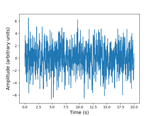
You cannot easily see the 0.5 s period in the light curve (this is also true if you zoom in), due to the large amplitude of noise added to the signal. Instead, let’s calculate the FFT of the signal, and from this measure the power, which is the modulus-squared of the complex amplitude of the FFT, and scales with the variance contributed to the time-series at each frequency. The resulting plot of power vs. frequency is called a power spectrum, also referred to as a periodogram when used to look for periodic signals, which will show up as a peak at a particular frequency.
Formally the scipy 1-D FFT function scipy.fft.fft calculates the so-called Discrete Fourier
Transform (DFT) \(y[k]\) of a contiguous time-series (i.e. measurements contained in equal time bins, with one measurement right after another with no gaps between bins).
For a time-series \(x[n]\) of length \(N\), \(y[k]\) is defined as:
[y[k] = \sum\limits^{N-1}_{n=0} x[n] \exp\left(-2\pi ikn/N \right)]
where \(k\) denotes the frequency bin (and \(i\) is the imaginary unit). The zero frequency bin
has an amplitude equal to the sum over all the \(x[n]\) values. Formally, \(k\) takes both
negative and positive values, extending to \(\pm \frac{N}{2}\) (the so-called Nyquist frequency).
However, for real-valued
time-series the negative frequency values are just the complex conjugates of the
corresponding positive-frequency values, so the convention is to only plot the positive frequencies.
It’s important to note however that the results of the scipy.fft.fft function are ‘packed’ in the
resulting DFT array so that for even \(N\), the elements \(y[1]...y[N/2-1]\) contain the positive
frequency terms
(in ascending frequency order) while elements \(y[N/2]...y[N-1]\) contain the negative frequency
terms (in order of decreasing absolute frequency).
Since the DFT does not take any time units, the actual frequencies \(f[k]\) may be calculated separately
(e.g. using the scipy.fft.fftfreq function). They can also be easily calculated by hand,
since they are simply related to \(k\) and the duration of the
time-series via \(f[k]=k/(N\Delta t)\) where \(\Delta t\) is the time step corresponding to one
time-series bin. Thus, the Nyquist frequency corresponds to \(f[N/2] = 1/(2\Delta t)\) and
only depends on the bin size.
Now that we know what scipy’s FFT function will give us, let’s calculate it for our noisy sinusoidal signal.
from scipy import fft

# The FFT of the signal
sig_fft = fft.fft(sig)

# And the power (sig_fft is of complex dtype), power is the modulus-squared of the FT
power = np.abs(sig_fft)**2

# The corresponding frequencies
sample_freq = fft.fftfreq(sig.size, d=time_step)

# Plot the FFT power, we only plot +ve frequencies (for real time series, -ve frequencies are
# complex conjugate of +ve). Note that if we don't restrict the index range to sig.size//2,
# the line plotting the power spectrum will wrap around to the negative value of the Nyquist frequency
plt.figure()
plt.plot(sample_freq[:sig.size//2], power[:sig.size//2])
plt.xlim(0,26.)
plt.xlabel('Frequency [Hz]',fontsize=14)
plt.ylabel('Power',fontsize=14)
plt.show()
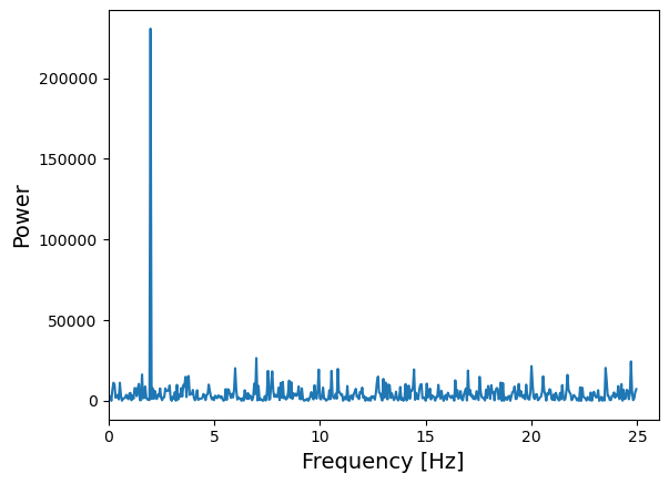
The sinusoidal signal at 2 Hz frequency is very clear in the power spectrum.
fft can also be given a multi-dimensional array as input, so that it will measure multiple FFTs
along a given axis (the last axis is used as a default). This can be used when multiple FFTs of
equal-length segments
of a time-series need to be calculated quickly (instead of repeatedly looping over the fft function).
Besides the FFT functions in scipy, numpy also contains a suite of FFT functions (in numpy.fft).
When searching for periodic signals against a background of white noise (random variations which
are statistically independent from one to the next), the scipy and numpy functions are useful when
the time-series consists of contiguous bins. If there are gaps in the time-series however,
the related Lomb-Scargle periodogram can be used. It can be found in Astropy, in the timeseries analysis sub-package, as astropy.timeseries.LombScargle.
Key Points
Scipy sub-packages need to be individually loaded -
import scipyand then referring to the package name is not sufficient. Instead use, e.g.from scipy import fft.Specific functions can also be loaded separately such as
from scipy.interpolate import interp1d.For model fitting when errors are normally distributed you can use
scipy.optimize.curve_fit. For more general function minimization usescipy.optimize.minimizeBe careful with how Scipy’s Fast Fourier Transform results are ordered in the output arrays.
Always be careful to read the documentation for any Scipy sub-packages and functions to see how they work and what is assumed.
Introduction to Astropy
Overview
Teaching: 40 min
Exercises: 0 minQuestions
How can the Astropy library help me with astronomical calculations and tasks?
Objectives
Discover some of the capabilities of Astropy sub-packages.
See how some of the subpackages can be used for working with physical units and constants, cosmological calculations and observation planning.
Introducing Astropy
Astropy is a community-driven Python package containing many tools
and functions that are useful for doing
astronomy and astrophysics, from observation planning, data reduction and data analysis to
modelling and numerical calculations. The astropy core package is included in Anaconda.
in case you don’t have it you can install it via pip using pip install astropy and
if necessary you can update your Anaconda installation using conda update astropy.
The astropy core package is documented here and includes a range of sub-packages:
| Sub-package | Methods covered |
|---|---|
config |
Control parameters used in astropy or affiliated packages |
constants |
Physical and astrophysical constants |
convolution |
Convolution and filtering |
coordinates |
Astronomical coordinate systems |
cosmology |
Perform cosmological calculations |
io |
Input/output of different file formats (FITS, ASCII, VOTable, HDF5, YAML, ASDF, pickle) |
modeling |
Models and model fitting |
nddata |
N-dimensional data-sets |
samp |
Simple Application Messaging Protocol: allows different catalogues and image viewers to interact |
stats |
Astrostatistics tools |
table |
Storage and manipulation of heterogeneous data tables using numpy functionality |
time |
Time and dates |
timeseries |
Time-series analysis |
uncertainty |
Uncertainties and distributions |
units |
Assigning units to variables and carrying out dimensionally-correct calculations |
utils |
General-purpose utilities and functions |
visualization |
Data visualization |
wcs |
World Coordinate System |
Besides the core packages, astropy maintains a number of separate coordinated packages which you may need to install separately. These packages are maintained by the astropy package but they are either too large to be part of the core package, or started out as affiliated packages that became part of the astropy `ecosystem’ so that they need to be maintained directly by the project.
| Coordinated package | Methods covered |
|---|---|
astropy-healpix |
Pixelization of a sphere (used for astronomical surveys) |
astroquery |
Tools for querying online astronomical catalogues and other data sources |
ccdproc |
Basic CCD data reduction |
photutils |
Photometry and related image-processing tools |
regions |
Region handling to allow extraction or masking of data from specific regions of astronomical images |
reproject |
Image reprojection, e.g. for comparing and overlaying images which have different coordinate systems (e.g. Galactic vs. RA/Dec) |
specutils |
Analysis tools and data types for astronomical spectra |
Alongside the core and coordinated packages, there are a large number of astropy affiliated packages. These are maintained separately from the main astropy project, but their developers/maintainers agree to follow astropy’s interface standards and philosophy of interoperability. Affiliated packages include packages to help plan observations, calculate the effects of dust extinction on photometric and spectral observations, solve gravitational and galactic dynamics problems and analyse data from gamma-ray observatories. We won’t list them all here - you can find the complete list of all coordinated and affiliated packages here.
Units, Quantities and Constants
Astronomical quantities are often given in a variety of non-SI units. Besides the strange
negative-logarithmic flux units of magnitudes (originating in Ancient Greece), for historical reasons,
astronomers often work with cm and g instead of m and kg. There are also a wide range
of units for expressing important astrophysical quantities in more ‘manageable’ amounts,
such as the parsec (pc) or
Astronomical Unit (AU) for distance, the solar mass unit (M\(_{\odot}\)) or useful
composite units, such as the solar
luminosity (L\(_{\odot}\)). Calculations using different units, or converting between units, can
be made much easier using Astropy’s units sub-package.
In astropy.units a unit represents the physical unit itself, while a quantity corresponds to
a given value combined with the unit it is expressed in. For example:
import astropy.units as u

v = 30 * u.km/u.s

print(v) # print the quantity v
print(v.unit)  # print the units of v
print(v.value) # print the value of v (it has no units)
30.0 km / s
km / s
30.0
You can do mathematics with quantities, and convert from one set of units to another.
v2 = v + 1700*u.m/u.s
print(v2) # The new quantity has the units of the quantity from the first term in the sum

mass = 1500*u.kg

ke = 0.5*mass*v2**2  # Let's calculate the kinetic energy
print(ke) # Multiplication/division results in quantities in composite units

ke_J = ke.to(u.J) # It's easy to convert to different units
print(ke_J)  # And we get the kinetic energy in Joules

print((0.5*mass*v2**2).to(u.J)) # We can also do the conversion on the same line as the calculation

print((0.5*mass*v2**2).si) # And we can also convert to systems of units
31.7 km / s
753667.5 kg km2 / s2
753667500000.0 J
753667500000.0 J
753667500000.0 m N
It’s also simple to convert to new composite units:
print*v2.to(u.au/u.h) # Get v2 in units of AU per hour
0.000762845082393275 AU / h
If you want to obtain a dimensionless value, you can use the decompose method:
print(20*u.lyr/u.au)  # How many AUs is 20 light-years?
print((20*u.lyr/u.au).decompose())
20.0 lyr / AU
1264821.5416853256
Note that quantities can only perform calculations that are consistent with their dimensions. Trying to add a distance to a mass will give an error message!
You can also use units and quantities in array calculations:
import numpy as np

v2_arr = v + 2000.*np.random.normal(size=10)*u.m/u.s
mass_arr = np.linspace(1000,2000,10)*u.kg

ke_arr = (0.5*mass_arr*v2_arr**2).to(u.J)
print(ke_arr)
[4.47854216e+11 5.02927405e+11 6.74449284e+11 6.68575939e+11
6.42467967e+11 6.05588651e+11 7.38080377e+11 8.02363612e+11
8.99907525e+11 8.51669433e+11] J
The capabilities of Astropy units are even more useful when combined with the wide range
of constants available in the constants sub-package. For example, let’s calculate
a General Relativistic quantity, the gravitational
radius, for a mass of 1 Solar mass (gravitational radius \(R_{g} = GM/c^{2}\)):
from astropy.constants import G, c, M_sun
print(G,c,M_sun,"\n")  # Printing will give some data about the assumed constants

print("Calculating the gravitational radius for 1 solar mass:")

R_g = G*M_sun/c**2  # Calculate the gravitational radius for 1 solar mass
print(R_g.cgs)  # Default units of constants are SI We can easily convert our result

print(G.cgs*M_sun.cgs/c.cgs**2) # We can also convert constants to cgs
  Name   = Gravitational constant
  Value  = 6.6743e-11
  Uncertainty  = 1.5e-15
  Unit  = m3 / (kg s2)
  Reference = CODATA 2018   Name   = Speed of light in vacuum
  Value  = 299792458.0
  Uncertainty  = 0.0
  Unit  = m / s
  Reference = CODATA 2018   Name   = Solar mass
  Value  = 1.988409870698051e+30
  Uncertainty  = 4.468805426856864e+25
  Unit  = kg
  Reference = IAU 2015 Resolution B 3 + CODATA 2018

Calculating the gravitational radius for 1 solar mass
147662.5038050125 cm
147662.50380501247 cm
The Astropy documentation for units and constants lists all the available units and constants,
so you can calculate gravitational force in units of solar mass Angstrom per fortnight\(^{2}\) if you wish!
Challenge
The Stefan-Boltzmann law gives the intensity (emitted power per unit area) of a blackbody of temperature \(T\) as: \(I = \sigma_{\rm SB} T^{4}\). A blackbody spectrum peaks at a wavelength \(\lambda_{\rm peak} = b/T\), where \(b\) is Wien’s displacement constant.
By using
astropy.unitsand importing fromastropy.constantsonly the two constants \(\sigma_{\rm SB}\) and \(b\), calculate and print in a single line of code the peak wavelength (in Angstroms) of the blackbody emission from the sun. You may also usenumpy.piand can assume that the entire emission from the sun is emitted as a blackbody spectrum with a single temperature.Hint 1
The solar constants you need are also provided in
astropy.unitsHint 2
We must rearrange \(L_{\odot} = 4\pi R_{\odot}^2 I\), then apply the Stefan-Boltzmann and Wien’s displacement laws to get the wavelength.
Solution
from astropy.constants import sigma_sb, b_wien

print((b_wien/((u.L_sun/(sigma_sb*4*np.pi*u.R_sun**2))**0.25)).to(u.angstrom))
5020.391950178645 Angstrom
Cosmological Calculations
When observing or interpreting data from sources at cosmological distances, it’s necessary to
take account of the effects of the expanding universe on the appearance of objects,
due to both their recession velocity (and hence, redshift) and the effects of the expansion of
space-time. Such effects depend on the assumed cosmological model (often informed by
recent cosmological data) and can be calculated using the Astropy cosmology sub-package.
To get started, we need to specify a cosmological model and its parameters. For ease-of-use, these can correspond to a specific set of parameters which are the best estimates measured by either the WMAP or Planck microwave background survey missions, assuming a flat Lambda-CDM model (cold dark matter with dark energy represented by a cosmological constant).
The cosmological model functions include the method .H(z) which returns the value of the
Hubble constant \(H\) at redshift \(z\).
from astropy.cosmology import WMAP9 as cosmo
print(cosmo)
print("Hubble constant at z = 0, 3:",cosmo.H(0),",",cosmo.H(3),"\n")

from astropy.cosmology import Planck15 as cosmo
print(cosmo)
print("Hubble constant at z = 0, 3:",cosmo.H(0),",",cosmo.H(3))
FlatLambdaCDM(name="WMAP9", H0=69.3 km / (Mpc s), Om0=0.286, Tcmb0=2.725 K, Neff=3.04, m_nu=[0. 0. 0.] eV, Ob0=0.0463)
Hubble constant at z = 0, 3: 69.32 km / (Mpc s) , 302.72820545374975 km / (Mpc s)

FlatLambdaCDM(name="Planck15", H0=67.7 km / (Mpc s), Om0=0.307, Tcmb0=2.725 K, Neff=3.05, m_nu=[0.   0.   0.06] eV, Ob0=0.0486)
Hubble constant at z = 0, 3: 67.74 km / (Mpc s) , 306.56821664118934 km / (Mpc s)
Note that the parameters in cosmological models are Astropy quantities with defined units - the same goes for the values calculated by the cosmological functions.
It’s also possible to specify the parameters of the model. There are a number of base classes for doing this. They must be imported and then called to define the cosmological parameters, e.g.:
from astropy.cosmology import FlatLambdaCDM  # Flat Lambda-CDM model
# Specify non-default parameters - it's recommended (but not required) to assign
# units to these constants
cosmo = FlatLambdaCDM(H0=70 * u.km / u.s / u.Mpc, Tcmb0=2.725 * u.K, Om0=0.3)
print(cosmo)
print("Hubble constant at z = 0, 3:",cosmo.H(0),",",cosmo.H(3))
FlatLambdaCDM(H0=70 km / (Mpc s), Om0=0.3, Tcmb0=2.725 K, Neff=3.04, m_nu=[0. 0. 0.] eV, Ob0=None)
Hubble constant at z = 0, 3: 70.0 km / (Mpc s) , 312.4364259948698 km / (Mpc s)
There are a number of other classes, all based on an isotropic and homogeneous (Friedmann-Lemaitre-Robertson-Walker - FLRW) cosmology and different forms of dark energy.
We’ll assume the Planck15 cosmology for the remaining calculations. For example, we want to determine the age of the universe at a number of redshifts:
from astropy.cosmology import Planck15 as cosmo

ages = cosmo.age([0,1,2,3])
print(ages)
[13.7976159 5.86254925 3.28395377 2.14856925] Gyr
Or we could find the luminosity distance at given redshifts (the effective distance for calculating the observed flux from an object using the inverse-square law). For example, an X-ray instrument measures X-ray fluxes (in cgs units) for 3 quasars with known redshifts, which we want to convert to luminosities:
z = [0.7,4.0,2.0]  # Quasar redshifts
flux_xray = [2.3e-12,3e-13,5.5e-13] * u.erg/(u.cm**2 * u.s) # We need to give correct units
print("X-ray fluxes =",flux_xray)

lum_dist = cosmo.luminosity_distance(z)
print("Luminosity distances = ",lum_dist)

lum_xray = flux_xray * 4*np.pi*lum_dist.to(u.cm)**2
print("X-ray luminosities = ",lum_xray)
X-ray fluxes = [2.3e-12 3.0e-13 5.5e-13] erg / (cm2 s)
Luminosity distances =  [ 4383.73875509 36697.036387   15934.6156438 ] Mpc
X-ray luminosities =  [5.28844656e+45 4.83386140e+46 1.67092451e+46] erg / s
Observation Planning
Astropy has a number of useful functions to allow the planning of observations from the ground. For example, suppose we want to observe the star Fomalhaut from one of the VLT telescopes in Paranal, Chile. We want to work out when Fomalhaut will be visible from Paranal and how high in the sky it will be, to find out when we can observe it with the minimum air-mass along the line of sight.
from astropy.coordinates import SkyCoord, EarthLocation, AltAz

# Lets observe the star Fomalhaut with the ESO VLT - 8m Telescope in Chile
# Load the position of Fomalhaut from the Simbad database

fomalhaut = SkyCoord.from_name('Fomalhaut')

print("Sky coordinates of Fomalhaut:",fomalhaut)

# Load the position of the Observatory. Physical units should be assigned via the
# units function
paranal = EarthLocation(lat=-24.62*u.deg, lon=-70.40*u.deg, height=2635*u.m)

print("Geocentric coordinates for Paranal: ",paranal)  # The coordinates are stored as geocentric (position
# relative to earth centre-of-mass) as a default
Sky coordinates of Fomalhaut: <SkyCoord (ICRS): (ra, dec) in deg
    (344.41269272, -29.62223703)>
Geocentric coordinates for Paranal:  (1946985.07871218, -5467769.32727434, -2641964.6140713) m
Now let’s say that we want to observe Fomalhaut and have been assigned observing time on the night of Oct 14 2020. We will determine the position in the sky as seen from Paranal over a 24 hour window centred on local midnight on that night. Note that a given date starts at 00:00:00, so the date we need is Oct 15 2020.
from astropy.time import Time

midnight = Time('2020-10-15 00:00:00')
# Define grid of times to calculate position over:
delta_midnight = np.linspace(-12, 12, 1000)*u.hour

times_Oct14_to_15 = midnight + delta_midnight

# Set up AltAz reference frame for these times and location
frame_Oct14_to_15 = AltAz(obstime=times_Oct14_to_15, location=paranal)

# Now we transform the Fomalhaut object to the Altitute/Azimuth coordinate system

fomalhaut_altazs_Oct14_to_15 = fomalhaut.transform_to(frame_Oct14_to_15)
We should also check the position of the sun in the Paranal sky over the same times (since this will determine whether the source is visible at night-time from this location):
from astropy.coordinates import get_sun

sunaltazs_Oct14_to_15 = get_sun(times_Oct14_to_15).transform_to(frame_Oct14_to_15)
Finally, we can plot the night-time observability of Fomalhaut from Paranal over this time range.
We will import and use an Astropy matplotlib style file from astropy.visualization in order to
make the plot look nicer (specifically, it will add a useful grid to the plot).
import matplotlib.pyplot as plt

from astropy.visualization import astropy_mpl_style
plt.style.use(astropy_mpl_style)

plt.figure()
# Plot the sun altitude
plt.plot(delta_midnight, sunaltazs_Oct14_to_15.alt, color='r', label='Sun')
# Plot Fomalhaut's alt/az - use a colour map to represent azimuth
plt.scatter(delta_midnight, fomalhaut_altazs_Oct14_to_15.alt,
            c=fomalhaut_altazs_Oct14_to_15.az, label='Fomalhaut', lw=0, s=8,
            cmap='viridis')
# Now plot the range when the sun is below the horizon, and at least 18 degrees below
# the horizon - this shows the range of twilight (-0 to -18 deg) and night (< -18 deg)
plt.fill_between(delta_midnight.to('hr').value, 0, 90,
                 sunaltazs_Oct14_to_15.alt < -0*u.deg, color='0.7', zorder=0)
plt.fill_between(delta_midnight.to('hr').value, 0, 90,
                 sunaltazs_Oct14_to_15.alt < -18*u.deg, color='0.4', zorder=0)
plt.colorbar().set_label('Azimuth [deg]')
plt.legend(loc='upper left')
plt.xlim(-12, 12)
plt.xticks(np.arange(13)*2 -12)
plt.ylim(0, 90)
plt.xlabel('Hours from UT Midnight')
plt.ylabel('Altitude [deg]')
plt.savefig('Fomalhaut_from_Paranal')
plt.show()
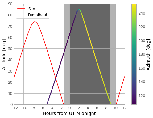
The colour scale shows the range of azimuthal angles of Fomalhaut. Twilight is represented by the light-grey shaded region, while night is the dark-grey shaded region. The plot shows that Fomalhaut is high in the Paranal sky earlier in local night-time, so should be observed in the first few hours of the night for optimum data-quality (since greater azimuth means lower air-mass along the line of sight to the target).
Key Points
Astropy includes the core packages plus coordinated sub-packages and affiliated sub-packages (which need to be installed separately).
The
astropy.unitssub-package enables calculations to be carried out using self-consistent physical units.
astropy.constantsenables calculations using physical constants using a whole range of physical units when combined with theunitssub-package.
astropy.cosmologyallows calculations of fundamental cosmological quantities such as the cosmological age or luminosity distance, for a specified cosmological model.
astropy.coordinatesandastropy.time, provide a number of functions that can be combined to determine when a given target object can best be observed from a given location.
Working with FITS Data
Overview
Teaching: 30 min
Exercises: 0 minQuestions
How do I access the data in FITS files?
Objectives
Understand how a FITS file is structured and how to determine the contents of a FITS file.
Print and access keyword information in FITS headers.
Read FITS data tables and read and plot FITS image data.
FITS File Structure
The Flexible Image Transport System (FITS) is a digital file format which
can be used to efficiently store tables or multi-dimensional data arrays, such as 2-D images. It was
designed for astronomical data, so it includes many features optimised for use with
such data, and is the most common digital file format in use in astronomy. The
astropy.io.fits sub-package allows you to read, manipulate and write FITS formatted data, so
that in combination with other Python and Astropy functions you can easily work with and analyse
astronomical data.
FITS files are organised in a particular way:
- Header Data Units (HDUs) are the highest-level component of a FITS file, consisting of a header and some type of data, which may be a table or a multi-dimensional data-array such as an image. The header contains the ‘metadata’ which describes the associated data.
- A FITS file may consist of multiple HDUs, the first of which is the primary HDU, followed by extensions denoted by an integer starting from 1. The primary HDU is listed as extension 0.
In this episode we will look at how to use astropy.io.fits to determine the structure and contents of FITS
files, and how to read in data and metadata (‘header’ information) from them. It is also possible to write
new FITS files, or edit existing ones. We will not describe this here but you can find out more via the official
documentation for astropy.io.fits here.
Let’s take a look at the FITS table file associated with this Episode, gal_info_dr7_v5_2.fit (you can download it here). This file
contains a large table of data for more than 900 000 galaxies observed as part of the Sloan
Digital Sky Survey (SDSS). First we will open the file and look at it’s
HDU structure:
from astropy.io import fits

gals = fits.open('gal_info_dr7_v5_2.fit')
gals.info()
Filename: gal_info_dr7_v5_2.fit
No.    Name      Ver    Type      Cards   Dimensions   Format
  0  PRIMARY       1 PrimaryHDU       4   ()
  1                1 BinTableHDU     67   927552R x 25C   [I, J, I, 5I, E, E, 5E, I, I, 19A, 6A, 21A, E, E, I, E, E, E, E, E, E, 3E, 3E, 5E, 12A]
We can see that the file consists of two HDUs, the primary (which in this case has no data attached)
and a table (which consists of 927552 rows and
25 columns). The Cards value lists the quantity of card images which make up the header for the HDU
and consist of a keyword name, a value and an optional) comment. Before we move on, we’ll take a
look at the header of the primary HDU, HDU[0], which consists of 4 cards:
gals[0].header
SIMPLE  =                    T /Dummy Created by MWRFITS v1.6a
BITPIX  =                    8 /Dummy primary header created by MWRFITS
NAXIS   =                    0 /No data is associated with this header
EXTEND  =                    T /Extensions may (will!) be present
For this particular file, the primary header is just a standard placeholder, which needs to be present but doesn’t convey any useful information. Other types of FITS data file may contain more extensive primary headers, e.g. containing important information about the observation (telescope, date, sky location) used to take an image or spectrum.
In case you want to look at the value or comment associated with a keyword:
print(gals[0].header['BITPIX'])
print(gals[0].header.comments['BITPIX'])
8
Dummy primary header created by MWRFITS
Returning to our list of HDUs, we see that HDU[1] has a more extensive header (with 67 cards) and a set of dimensions (927552 rows and 25 columns) and data formats corresponding to the table dimensions and the formats of the data in the columns therein.
Working with FITS Table Extensions
Now we’ll look at the table extension HDU[1], which contains the data. It’s useful first to look at the names
and formats of the columns we have, using the .columns method:
gals[1].columns
ColDefs(
    name = 'PLATEID'; format = 'I'
    name = 'MJD'; format = 'J'
    name = 'FIBERID'; format = 'I'
    name = 'PHOTOID'; format = '5I'
    name = 'RA'; format = 'E'
    name = 'DEC'; format = 'E'
    name = 'PLUG_MAG'; format = '5E'
    name = 'PRIMTARGET'; format = 'I'
    name = 'SECTARGET'; format = 'I'
    name = 'TARGETTYPE'; format = '19A'
    name = 'SPECTROTYPE'; format = '6A'
    name = 'SUBCLASS'; format = '21A'
    name = 'Z'; format = 'E'
    name = 'Z_ERR'; format = 'E'
    name = 'Z_WARNING'; format = 'I'
    name = 'V_DISP'; format = 'E'
    name = 'V_DISP_ERR'; format = 'E'
    name = 'SN_MEDIAN'; format = 'E'
    name = 'E_BV_SFD'; format = 'E'
    name = 'ZTWEAK'; format = 'E'
    name = 'ZTWEAK_ERR'; format = 'E'
    name = 'SPECTRO_MAG'; format = '3E'
    name = 'KCOR_MAG'; format = '3E'
    name = 'KCOR_MODEL_MAG'; format = '5E'
    name = 'RELEASE'; format = '12A'
)
The formats I, J, E and A denote respectively: 16-bit integers, 32-bit integers, single-precision floats and
characters
(i.e. single elements from a string). The digits N in front of a letter format identifier show that that quantity is
an array with N elements (if an integer or float) or a string with N characters. (note that short descriptions
of the column data are given on the SDSS galaxy data webpage
here).
To access the table data itself, we use the .data method:
gal_data = gals[1].data
The resulting array gal_data is a numpy record_array: a type of structured array that can have its columns indexed either with their field name (which is simply the column name) or by giving the field name as an attribute (suffix after the record array name). E.g., to use both approaches to print out the redshifts:
print(gal_data['Z'])
print(gal_data.Z)
[0.02127545 0.21392463 0.12655362 ... 0.16735837 0.11154801 0.22395724]
[0.02127545 0.21392463 0.12655362 ... 0.16735837 0.11154801 0.22395724]
The usual indexing and slicing can then be used to access the rows of the column, e.g.:
print(gal_data.Z[20:25])
[0.1314682 0.00628221 0.04809635 0.08410355 0.09024068]
Printing a specific item for one of the quantities that is listed as an array type, will give an array:
print(gal_data.KCOR_MAG[10])
[18.97718 18.35391 18.052666]
Plotting an image from a FITS file
Image data in FITS files takes the form of a 2-dimensional array where each item corresponds to a pixel value.
For example, let’s look at a FITS image of the famous Horsehead nebula. You can find it in the Lesson
data directory here). We’ll first open the file and look at
its structure:
horsehead = fits.open('HorseHead.fits')
horsehead.info()
Filename: HorseHead.fits
No.    Name      Ver    Type      Cards   Dimensions   Format
  0  PRIMARY       1 PrimaryHDU     161   (891, 893)   int16
  1  er.mask       1 TableHDU        25   1600R x 4C   [F6.2, F6.2, F6.2, F6.2]
The image here (with dimensions 891\(\times\)893 pixels) is in the primary HDU (HDU[0]), while HDU[1] is a
table with 1600 rows and 4 columns (we won’t consider this table further here). To plot the image, we can use
the special matplotlib function imshow, which is designed to plot values from 2-D arrays as an image,
using a colour map to denote each value. We will assume a basic grey colour map here, but a wide range
of different colour maps are
available (you can check the matplotlib documentation for details). To indicate how values map on to the
colour map, we also include a colour bar with the plot.
import matplotlib.pyplot as plt

image_data = horsehead[0].data # Get the data associated with the HDU, same as for a table

plt.figure()
plt.imshow(image_data, cmap='gray')
plt.colorbar()
plt.show()

The image is plotted in terms of the pixel position on the \(x\) and \(y\) axes. Astropy contains a range of functions for plotting images in actual sky coordinates, overlaying coordinate grids, contours etc. (e.g. see the documentation for the astropy.wcs and astropy.visualization sub-packages).
Key Points
FITS files can be read in and explored using the
astropy.io.fitssub-package. Theopencommand is used to open a datafile.FITS files consist of one or more Header Data Units (HDUs) which include a header and possibly data, in the form of a table or image. The structure can be accessed using the
.info()methodHeaders contain sets of keyword/value pairs (like a dictionary) and optional comments, which describe the metadata for the data set, accessible using the
.header['KEYWORD']method.Tables and images can be accessed using the
.datamethod, which assigns table data to a structured array, while image data is assigned to an n-dimensional array which may be plotted with e.g. matplotlib’simshowfunction.