Introduction to Astropy

Overview

Teaching: 40 min
Exercises: 0 min

Questions

• How can the Astropy library help me with astronomical calculations and tasks?

Objectives

• Discover some of the capabilities of Astropy sub-packages.

• See how some of the subpackages can be used for working with physical units and constants, cosmological calculations and observation planning.

Introducing Astropy

Astropy is a community-driven Python package containing many tools and functions that are useful for doing astronomy and astrophysics, from observation planning, data reduction and data analysis to modelling and numerical calculations. The astropy core package is included in Anaconda. in case you don’t have it you can install it via pip using pip install astropy and if necessary you can update your Anaconda installation using conda update astropy.

The astropy core package is documented here and includes a range of sub-packages:

Besides the core packages, astropy maintains a number of separate coordinated packages which you may need to install separately. These packages are maintained by the astropy package but they are either too large to be part of the core package, or started out as affiliated packages that became part of the astropy `ecosystem’ so that they need to be maintained directly by the project.

Alongside the core and coordinated packages, there are a large number of astropy affiliated packages. These are maintained separately from the main astropy project, but their developers/maintainers agree to follow astropy’s interface standards and philosophy of interoperability. Affiliated packages include packages to help plan observations, calculate the effects of dust extinction on photometric and spectral observations, solve gravitational and galactic dynamics problems and analyse data from gamma-ray observatories. We won’t list them all here - you can find the complete list of all coordinated and affiliated packages here.

Units, Quantities and Constants

Astronomical quantities are often given in a variety of non-SI units. Besides the strange negative-logarithmic flux units of magnitudes (originating in Ancient Greece), for historical reasons, astronomers often work with cm and g instead of m and kg. There are also a wide range of units for expressing important astrophysical quantities in more ‘manageable’ amounts, such as the parsec (pc) or Astronomical Unit (AU) for distance, the solar mass unit (M\(_{\odot}\)) or useful composite units, such as the solar luminosity (L\(_{\odot}\)). Calculations using different units, or converting between units, can be made much easier using Astropy’s units sub-package.

In astropy.units a unit represents the physical unit itself, while a quantity corresponds to a given value combined with the unit it is expressed in. For example:

import astropy.units as u

v = 30 * u.km/u.s

print(v) # print the quantity v
print(v.unit)  # print the units of v
print(v.value) # print the value of v (it has no units)

30.0 km / s
km / s
30.0

You can do mathematics with quantities, and convert from one set of units to another.

v2 = v + 1700*u.m/u.s 
print(v2) # The new quantity has the units of the quantity from the first term in the sum

mass = 1500*u.kg 

ke = 0.5*mass*v2**2  # Let's calculate the kinetic energy
print(ke) # Multiplication/division results in quantities in composite units

ke_J = ke.to(u.J) # It's easy to convert to different units
print(ke_J)  # And we get the kinetic energy in Joules

print((0.5*mass*v2**2).to(u.J)) # We can also do the conversion on the same line as the calculation

print((0.5*mass*v2**2).si) # And we can also convert to systems of units

31.7 km / s
753667.5 kg km2 / s2
753667500000.0 J
753667500000.0 J
753667500000.0 m N

It’s also simple to convert to new composite units:

print*v2.to(u.au/u.h)  # Get v2 in units of AU per hour

0.000762845082393275 AU / h

If you want to obtain a dimensionless value, you can use the decompose method:

print(20*u.lyr/u.au)  # How many AUs is 20 light-years?
print((20*u.lyr/u.au).decompose())

20.0 lyr / AU
1264821.5416853256

Note that quantities can only perform calculations that are consistent with their dimensions. Trying to add a distance to a mass will give an error message!

You can also use units and quantities in array calculations:

import numpy as np

v2_arr = v + 2000.*np.random.normal(size=10)*u.m/u.s
mass_arr = np.linspace(1000,2000,10)*u.kg

ke_arr = (0.5*mass_arr*v2_arr**2).to(u.J)
print(ke_arr)

[4.47854216e+11 5.02927405e+11 6.74449284e+11 6.68575939e+11
6.42467967e+11 6.05588651e+11 7.38080377e+11 8.02363612e+11
8.99907525e+11 8.51669433e+11] J

The capabilities of Astropy units are even more useful when combined with the wide range of constants available in the constants sub-package. For example, let’s calculate a General Relativistic quantity, the gravitational radius, for a mass of 1 Solar mass (gravitational radius \(R_{g} = GM/c^{2}\)):

from astropy.constants import G, c, M_sun
print(G,c,M_sun,"\n")  # Printing will give some data about the assumed constants

print("Calculating the gravitational radius for 1 solar mass:")

R_g = G*M_sun/c**2  # Calculate the gravitational radius for 1 solar mass
print(R_g.cgs)  # Default units of constants are SI We can easily convert our result

print(G.cgs*M_sun.cgs/c.cgs**2) # We can also convert constants to cgs

  Name   = Gravitational constant
  Value  = 6.6743e-11
  Uncertainty  = 1.5e-15
  Unit  = m3 / (kg s2)
  Reference = CODATA 2018   Name   = Speed of light in vacuum
  Value  = 299792458.0
  Uncertainty  = 0.0
  Unit  = m / s
  Reference = CODATA 2018   Name   = Solar mass
  Value  = 1.988409870698051e+30
  Uncertainty  = 4.468805426856864e+25
  Unit  = kg
  Reference = IAU 2015 Resolution B 3 + CODATA 2018 

Calculating the gravitational radius for 1 solar mass
147662.5038050125 cm
147662.50380501247 cm

The Astropy documentation for units and constants lists all the available units and constants, so you can calculate gravitational force in units of solar mass Angstrom per fortnight\(^{2}\) if you wish!

Challenge

The Stefan-Boltzmann law gives the intensity (emitted power per unit area) of a blackbody of temperature \(T\) as: \(I = \sigma_{\rm SB} T^{4}\). A blackbody spectrum peaks at a wavelength \(\lambda_{\rm peak} = b/T\), where \(b\) is Wien’s displacement constant.

By using astropy.units and importing from astropy.constants only the two constants \(\sigma_{\rm SB}\) and \(b\), calculate and print in a single line of code the peak wavelength (in Angstroms) of the blackbody emission from the sun. You may also use numpy.pi and can assume that the entire emission from the sun is emitted as a blackbody spectrum with a single temperature.

Hint 1

The solar constants you need are also provided in astropy.units

Hint 2

We must rearrange \(L_{\odot} = 4\pi R_{\odot}^2 I\), then apply the Stefan-Boltzmann and Wien’s displacement laws to get the wavelength.

Solution

from astropy.constants import sigma_sb, b_wien

print((b_wien/((u.L_sun/(sigma_sb*4*np.pi*u.R_sun**2))**0.25)).to(u.angstrom))

5020.391950178645 Angstrom 

Cosmological Calculations

When observing or interpreting data from sources at cosmological distances, it’s necessary to take account of the effects of the expanding universe on the appearance of objects, due to both their recession velocity (and hence, redshift) and the effects of the expansion of space-time. Such effects depend on the assumed cosmological model (often informed by recent cosmological data) and can be calculated using the Astropy cosmology sub-package.

To get started, we need to specify a cosmological model and its parameters. For ease-of-use, these can correspond to a specific set of parameters which are the best estimates measured by either the WMAP or Planck microwave background survey missions, assuming a flat Lambda-CDM model (cold dark matter with dark energy represented by a cosmological constant). The cosmological model functions include the method .H(z) which returns the value of the Hubble constant \(H\) at redshift \(z\).

from astropy.cosmology import WMAP9 as cosmo
print(cosmo)
print("Hubble constant at z = 0, 3:",cosmo.H(0),",",cosmo.H(3),"\n")

from astropy.cosmology import Planck15 as cosmo
print(cosmo)
print("Hubble constant at z = 0, 3:",cosmo.H(0),",",cosmo.H(3))

FlatLambdaCDM(name="WMAP9", H0=69.3 km / (Mpc s), Om0=0.286, Tcmb0=2.725 K, Neff=3.04, m_nu=[0. 0. 0.] eV, Ob0=0.0463)
Hubble constant at z = 0, 3: 69.32 km / (Mpc s) , 302.72820545374975 km / (Mpc s) 

FlatLambdaCDM(name="Planck15", H0=67.7 km / (Mpc s), Om0=0.307, Tcmb0=2.725 K, Neff=3.05, m_nu=[0.   0.   0.06] eV, Ob0=0.0486)
Hubble constant at z = 0, 3: 67.74 km / (Mpc s) , 306.56821664118934 km / (Mpc s)

Note that the parameters in cosmological models are Astropy quantities with defined units - the same goes for the values calculated by the cosmological functions.

It’s also possible to specify the parameters of the model. There are a number of base classes for doing this. They must be imported and then called to define the cosmological parameters, e.g.:

from astropy.cosmology import FlatLambdaCDM  # Flat Lambda-CDM model
# Specify non-default parameters - it's recommended (but not required) to assign
# units to these constants
cosmo = FlatLambdaCDM(H0=70 * u.km / u.s / u.Mpc, Tcmb0=2.725 * u.K, Om0=0.3) 
print(cosmo) 
print("Hubble constant at z = 0, 3:",cosmo.H(0),",",cosmo.H(3))

FlatLambdaCDM(H0=70 km / (Mpc s), Om0=0.3, Tcmb0=2.725 K, Neff=3.04, m_nu=[0. 0. 0.] eV, Ob0=None)
Hubble constant at z = 0, 3: 70.0 km / (Mpc s) , 312.4364259948698 km / (Mpc s)

There are a number of other classes, all based on an isotropic and homogeneous (Friedmann-Lemaitre-Robertson-Walker - FLRW) cosmology and different forms of dark energy.

We’ll assume the Planck15 cosmology for the remaining calculations. For example, we want to determine the age of the universe at a number of redshifts:

from astropy.cosmology import Planck15 as cosmo

ages = cosmo.age([0,1,2,3])
print(ages)

[13.7976159   5.86254925  3.28395377  2.14856925] Gyr

Or we could find the luminosity distance at given redshifts (the effective distance for calculating the observed flux from an object using the inverse-square law). For example, an X-ray instrument measures X-ray fluxes (in cgs units) for 3 quasars with known redshifts, which we want to convert to luminosities:

z = [0.7,4.0,2.0]  # Quasar redshifts
flux_xray = [2.3e-12,3e-13,5.5e-13] * u.erg/(u.cm**2 * u.s) # We need to give correct units
print("X-ray fluxes =",flux_xray)

lum_dist = cosmo.luminosity_distance(z)
print("Luminosity distances = ",lum_dist)

lum_xray = flux_xray * 4*np.pi*lum_dist.to(u.cm)**2
print("X-ray luminosities = ",lum_xray)

X-ray fluxes = [2.3e-12 3.0e-13 5.5e-13] erg / (cm2 s)
Luminosity distances =  [ 4383.73875509 36697.036387   15934.6156438 ] Mpc
X-ray luminosities =  [5.28844656e+45 4.83386140e+46 1.67092451e+46] erg / s

Observation Planning

Astropy has a number of useful functions to allow the planning of observations from the ground. For example, suppose we want to observe the star Fomalhaut from one of the VLT telescopes in Paranal, Chile. We want to work out when Fomalhaut will be visible from Paranal and how high in the sky it will be, to find out when we can observe it with the minimum air-mass along the line of sight.

from astropy.coordinates import SkyCoord, EarthLocation, AltAz

# Lets observe the star Fomalhaut with the ESO VLT - 8m Telescope in Chile
# Load the position of Fomalhaut from the Simbad database

fomalhaut = SkyCoord.from_name('Fomalhaut')

print("Sky coordinates of Fomalhaut:",fomalhaut)

# Load the position of the Observatory. Physical units should be assigned via the
# units function
paranal = EarthLocation(lat=-24.62*u.deg, lon=-70.40*u.deg, height=2635*u.m) 

print("Geocentric coordinates for Paranal: ",paranal)  # The coordinates are stored as geocentric (position
# relative to earth centre-of-mass) as a default

Sky coordinates of Fomalhaut: <SkyCoord (ICRS): (ra, dec) in deg
    (344.41269272, -29.62223703)>
Geocentric coordinates for Paranal:  (1946985.07871218, -5467769.32727434, -2641964.6140713) m

Now let’s say that we want to observe Fomalhaut and have been assigned observing time on the night of Oct 14 2020. We will determine the position in the sky as seen from Paranal over a 24 hour window centred on local midnight on that night. Note that a given date starts at 00:00:00, so the date we need is Oct 15 2020.

from astropy.time import Time

midnight = Time('2020-10-15 00:00:00')
# Define grid of times to calculate position over:
delta_midnight = np.linspace(-12, 12, 1000)*u.hour 

times_Oct14_to_15 = midnight + delta_midnight

# Set up AltAz reference frame for these times and location
frame_Oct14_to_15 = AltAz(obstime=times_Oct14_to_15, location=paranal)

# Now we transform the Fomalhaut object to the Altitute/Azimuth coordinate system

fomalhaut_altazs_Oct14_to_15 = fomalhaut.transform_to(frame_Oct14_to_15)

We should also check the position of the sun in the Paranal sky over the same times (since this will determine whether the source is visible at night-time from this location):

from astropy.coordinates import get_sun

sunaltazs_Oct14_to_15 = get_sun(times_Oct14_to_15).transform_to(frame_Oct14_to_15)

Finally, we can plot the night-time observability of Fomalhaut from Paranal over this time range. We will import and use an Astropy matplotlib style file from astropy.visualization in order to make the plot look nicer (specifically, it will add a useful grid to the plot).

import matplotlib.pyplot as plt

from astropy.visualization import astropy_mpl_style
plt.style.use(astropy_mpl_style)

plt.figure()
# Plot the sun altitude
plt.plot(delta_midnight, sunaltazs_Oct14_to_15.alt, color='r', label='Sun')
# Plot Fomalhaut's alt/az - use a colour map to represent azimuth
plt.scatter(delta_midnight, fomalhaut_altazs_Oct14_to_15.alt, 
            c=fomalhaut_altazs_Oct14_to_15.az, label='Fomalhaut', lw=0, s=8,
            cmap='viridis')
# Now plot the range when the sun is below the horizon, and at least 18 degrees below 
# the horizon - this shows the range of twilight (-0 to -18 deg) and night (< -18 deg)
plt.fill_between(delta_midnight.to('hr').value, 0, 90,
                 sunaltazs_Oct14_to_15.alt < -0*u.deg, color='0.7', zorder=0)
plt.fill_between(delta_midnight.to('hr').value, 0, 90,
                 sunaltazs_Oct14_to_15.alt < -18*u.deg, color='0.4', zorder=0)
plt.colorbar().set_label('Azimuth [deg]')
plt.legend(loc='upper left')
plt.xlim(-12, 12)
plt.xticks(np.arange(13)*2 -12)
plt.ylim(0, 90)
plt.xlabel('Hours from UT Midnight')
plt.ylabel('Altitude [deg]')
plt.savefig('Fomalhaut_from_Paranal')
plt.show()

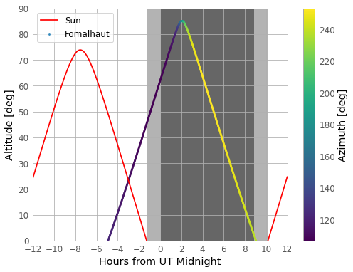
The colour scale shows the range of azimuthal angles of Fomalhaut. Twilight is represented by the light-grey shaded region, while night is the dark-grey shaded region. The plot shows that Fomalhaut is high in the Paranal sky earlier in local night-time, so should be observed in the first few hours of the night for optimum data-quality (since greater azimuth means lower air-mass along the line of sight to the target).

Key Points

• Astropy includes the core packages plus coordinated sub-packages and affiliated sub-packages (which need to be installed separately).

• The astropy.units sub-package enables calculations to be carried out using self-consistent physical units.

• astropy.constants enables calculations using physical constants using a whole range of physical units when combined with the units sub-package.

• astropy.cosmology allows calculations of fundamental cosmological quantities such as the cosmological age or luminosity distance, for a specified cosmological model.

• astropy.coordinates and astropy.time, provide a number of functions that can be combined to determine when a given target object can best be observed from a given location.