Random variables

Overview

Teaching: 40 min
Exercises: 10 min

Questions

• How do I calculate the means, variances and other statistical quantities for numbers drawn from probability distributions?

• How is the error on a sample mean calculated?

Objectives

• Learn how the expected means and variances of random variables (and functions of them) can be calculated from their probability distributions.

• Discover the scipy.stats functionality for calculated statistical properties of probability distributions and how to generate random numbers from them.

• Learn how key results such as the standard error on the mean and Bessel’s correction are derived from the statistics of sums of random variables.

In this episode we will be using numpy, as well as matplotlib’s plotting library. Scipy contains an extensive range of distributions in its ‘scipy.stats’ module, so we will also need to import it. Remember: scipy modules should be installed separately as required - they cannot be called if only scipy is imported.

import numpy as np
import matplotlib.pyplot as plt
import scipy.stats as sps

So far we have introduced the idea of working with data which contains some random component (as well as a possible systematic error). We have also introduced the idea of probability distributions of random variables. In this episode we will start to make the connection between the two because all data, to some extent, is a collection of random variables. In order to understand how the data are distributed, what the sample properties such as mean and variance can tell us and how we can use our data to test hypotheses, we need to understand how collections of random variables behave.

Properties of random variables: expectation

Consider a set of random variables which are independent, which means that the outcome of one does not affect the probability of the outcome of another. The random variables are drawn from some probability distribution with pdf \(p(x)\).

The expectation \(E(X)\) is equal to the arithmetic mean of the random variables as the number of sampled variates (realisations of the variable sampled from its probability distribution) increases \(\rightarrow \infty\). For a continuous probability distribution it is given by the mean of the distribution function, i.e. the pdf:

This quantity \(\mu\) is often just called the mean of the distribution, or the population mean to distinguish it from the sample mean of data.

More generally, we can obtain the expectation of some function of \(X\), \(f(X)\):

It follows that the expectation is a linear operator. So we can also consider the expectation of a scaled sum of variables \(X_{1}\) and \(X_{2}\) (which may themselves have different distributions):

Properties of random variables: variance

The (population) variance of a discrete random variable \(X\) with (population) mean \(\mu\) is the expectation of the function that gives the squared difference from the mean:

It is possible to rearrange things:

\(V[X] = E[(X-\mu)^{2})] = E[X^{2}-2X\mu+\mu^{2}]\) \(\rightarrow V[X] = E[X^{2}] - E[2X\mu] + E[\mu^{2}] = E[X^{2}] - 2\mu^{2} + \mu^{2}\) \(\rightarrow V[X] = E[X^{2}] - \mu^{2} = E[X^{2}] - E[X]^{2}\)

In other words, the variance is the expectation of squares - square of expectations. Therefore, for a function of \(X\):

Means and variances of the uniform and normal distributions

The distribution of a random variable is given using the notation \(\sim\), meaning ‘is distributed as’. I.e. for \(X\) drawn from a uniform distribution over the interval \([a,b]\), we write \(X\sim U(a,b)\). For this case, we can use the approach given above to calculate the mean: \(E[X] = (b+a)/2\) and variance: \(V[X] = (b-a)^{2}/12\)

The scipy.stats distribution functions include methods to calculate the means and variances for a distribution and given parameters, which we can use to verify these results, e.g.:

## Assume a = 1, b = 8 (remember scale = b-a)
a, b = 1, 8
print("Mean is :",sps.uniform.mean(loc=a,scale=b-a))
print("analytical mean:",(b+a)/2)
## Now the variance
print("Variance is :",sps.uniform.var(loc=a,scale=b-a))
print("analytical variance:",((b-a)**2)/12)

Mean is : 4.5
analytical mean: 4.5
Variance is : 4.083333333333333
analytical variance: 4.083333333333333

For the normal distribution with parameters \(\mu\), \(\sigma\), \(X\sim N(\mu,\sigma)\), the results are very simple because \(E[X]=\mu\) and \(V[X]=\sigma^{2}\). E.g.

## Assume mu = 4, sigma = 3
print("Mean is :",sps.norm.mean(loc=4,scale=3))
print("Variance is :",sps.norm.var(loc=4,scale=3))

Mean is : 4.0
Variance is : 9.0

Generating random variables

So far we have discussed random variables in an abstract sense, in terms of the population, i.e. the continuous probability distribution. But real data is in the form of samples: individual measurements or collections of measurements, so we can get a lot more insight if we can generate ‘fake’ samples from a given distribution.

A random variate is the quantity that is generated while a random variable is the notional object able to assume different numerical values, i.e. the distinction is similar to the distinction in python between x=15 and the object to which the number is assigned x (the variable).

The scipy.stats distribution functions have a method rvs for generating random variates that are drawn from the distribution (with the given parameter values). You can either freeze the distribution or specify the parameters when you call it. The number of variates generated is set by the size argument and the results are returned to a numpy array.

# Generate 10 uniform variates from U(0,1) - the default loc and scale arguments
u_vars = sps.uniform.rvs(size=10)
print("Uniform variates generated:",u_vars)

# Generate 10 normal variates from N(20,3)
n_vars = sps.norm.rvs(loc=20,scale=3,size=10)
print("Normal variates generated:",n_vars)

Uniform variates generated: [0.99808848 0.9823057  0.01062957 0.80661773 0.02865487 0.18627394 0.87023007 0.14854033 0.19725284 0.45448424]
Normal variates generated: [20.35977673 17.66489157 22.43217609 21.39929951 18.87878728 18.59606091 22.51755213 21.43264709 13.87430417 23.95626361]

Remember that these numbers depend on the starting seed which is almost certainly unique to your computer (unless you pre-select it: see below). They will also change each time you run the code cell.

How random number generation works

Random number generators use algorithms which are strictly pseudo-random since (at least until quantum-computers become mainstream) no algorithm can produce genuinely random numbers. However, the non-randomness of the algorithms that exist is impossible to detect, even in very large samples.

For any distribution, the starting point is to generate uniform random variates in the interval \([0,1]\) (often the interval is half-open \([0,1)\), i.e. exactly 1 is excluded). \(U(0,1)\) is the same distribution as the distribution of percentiles - a fixed range quantile has the same probability of occurring wherever it is in the distribution, i.e. the range 0.9-0.91 has the same probability of occuring as 0.14-0.15. This means that by drawing a \(U(0,1)\) random variate to generate a quantile and putting that in the ppf of the distribution of choice, the generator can produce random variates from that distribution. All this work is done ‘under the hood’ within the scipy.stats distribution function.

It’s important to bear in mind that random variates work by starting from a ‘seed’ (usually an integer) and then each call to the function will generate a new (pseudo-)independent variate but the sequence of variates is replicated if you start with the same seed. However, seeds are generated by starting from a system seed set using random and continuously updated data in a special file in your computer, so they will differ each time you run the code.

You can force the seed to take a fixed (integer) value using the numpy.random.seed() function. It also works for the scipy.stats functions, which use numpy.random to generate their random numbers. Include your chosen seed value as a function argument - the sequence of random numbers generated will only change if you change the seed (but their mapping to the distribution - which is via the ppf - will mean that the values are different for different distributions). Use the function with no argument in order to reset back to the system seed.

Sums of random variables

Since the expectation of the sum of two scaled variables is the sum of the scaled expectations, we can go further and write the expectation for a scaled sum of variables \(Y=\sum\limits_{i=1}^{n} a_{i}X_{i}\):

What about the variance? We can first use the expression in terms of the expectations:

and convert to linear sums of expectations in terms of \(X_{i}\):

Of the four terms on the LHS, the squared terms only in \(i\) are equal to the summed variances while the cross-terms in \(i\) and \(j\) can be paired up to form the so-called covariances (which we will cover when we discuss bi- and multivariate statistics):

For independent random variables, the covariances (taken in the limit of an infinite number of trials, i.e. the expectations of the sample covariance) are equal to zero. Therefore, the expected variance is equal to the sum of the individual variances multiplied by their squared scaling factors:

Intuition builder: covariance of independent random variables

The covariant terms above disappear because for pairs of independent variables \(X_{i}\), \(X_{j}\) (where \(i \neq j\)), \(E[X_{i}X_{j}]=E[X_{i}]E[X_{j}]\). By generating many (\(N\)) pairs of independent random variables (from either the uniform or normal distribution), show that this equality is approached in the limit of large \(N\), by plotting a graph of the average of the absolute difference \(\lvert \langle X_{1}X_{2} \rangle - \langle X_{1} \rangle \langle X_{2} \rangle \rvert\) versus \(N\), where \(X_{1}\) and \(X_{2}\) are independent random numbers and angle-brackets denote sample means over the \(N\) pairs of random numbers. You will need to repeat the calculation many (e.g. at least 100) times to find the average for each \(N\), since there will be some random scatter in the absolute difference. To give a good range of \(N\), step through 10 to 20 values of \(N\) which are geometrically spaced from \(N=10\) to \(N=10^{5}\).

Hint

It will be much faster if you generate the values for \(X_{1}\) and \(X_{2}\) using numpy arrays of random variates, e.g.: x1 = sps.uniform.rvs(loc=3,scale=5,size=(100,N)) will produce 100 sets of \(N\) uniformly distributed random numbers. The multiplied arrays can be averaged over the \(N\) values using the axis=1 argument with np.mean, before being averaged again over the 100 (or more) sets.

Solution

ntrials = np.geomspace(10,1e5,20,dtype=int)
# Set up the array to record the differences
diff = np.zeros(len(ntrials))

for i, N in enumerate(ntrials):
    # E.g. generate uniform variates drawn from U[3,8]
    x1 = sps.uniform.rvs(loc=3,scale=5,size=(100,N))
    x2 = sps.uniform.rvs(loc=3,scale=5,size=(100,N))
    diff[i] = np.mean(np.abs(np.mean(x1*x2,axis=1)-np.mean(x1,axis=1)*np.mean(x2,axis=1)))
    
plt.figure()
plt.scatter(ntrials,diff)
# We should use a log scale because of the wide range in values on both axis
plt.xscale('log')
plt.yscale('log')
plt.xlabel('$N$',fontsize=14)
# We add an extra pair of angle brackets outside, since we are averaging again over the 100 sets
plt.ylabel(r'$\langle |\langle X_{1}X_{2} \rangle - \langle X_{1} \rangle \langle X_{2} \rangle|\rangle$',fontsize=14)
plt.show()

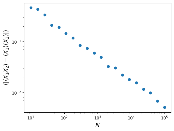
Note that the size of the residual difference between the product of averages and average of products scales as \(1/\sqrt{N}\).

The standard error on the mean

We’re now in a position to estimate the uncertainty on the mean of our speed-of-light data, since the sample mean is effectively equal to a sum of scaled random variables (our \(n\) individual measurements \(x_{i}\)):

The scaling factor is \(1/n\) which is the same for all \(i\). Now, the expectation of our sample mean (i.e. over an infinite number of trials, that is repeats of the same collection of 100 measurements) is:

Here we also implicitly assume that the measurements \(X_{i}\) are all drawn from the same (i.e. stationary) distribution, i.e \(E[x_{i}] = \mu\) for all \(i\). If this is the case, then in the absence of any systematic error we expect that \(\mu=c_{\mathrm{air}}\), the true value for the speed of light in air.

However, we don’t measure \(\mu\), which corresponds to the population mean!! We actually measure the scaled sum of measurements, i.e. the sample mean \(\bar{x}\), and this is distributed around the expectation value \(\mu\) with variance \(V[\bar{x}] = \sum\limits_{i=1}^{n} n^{-2} \sigma_{i}^{2} = \sigma^{2}/n\) (using the result for variance of a sum of random variables with scaling factor \(a_{i}=1/n\) assuming the measurements are all drawn from the same distribution, i.e. \(\sigma_{i}=\sigma\)). Therefore the expected standard deviation on the mean of \(n\) values, also known as the standard error is:

where \(\sigma\) is the population standard deviation. If we guess that the sample standard deviation is the same as that of the population (and we have not yet shown whether this is a valid assumption!), we estimate a standard error of 7.9 km/s for the 100 measurements, i.e. the observed sample mean is \(\sim19\) times the standard error away from the true value!

We have already made some progress, but we still cannot formally answer our question about whether the difference of our sample mean from \(c_{\mathrm{air}}\) is real or due to statistical error. This is for two reasons:

1. The standard error on the sample mean assumes that we know the population standard deviation. This is not the same as the sample standard deviation, although we might expect it to be similar.
2. Even assuming that we know the standard deviation and mean of the population of sample means, we don’t know what the distribution of that population is yet, i.e. we don’t know the probability distribution of our sample mean.

We will address these remaining issues in the next episodes.

Estimators, bias and Bessel’s correction

An estimator is a method for calculating from data an estimate of a given quantity. The results of biased estimators may be systematically biased away from the true value they are trying to estimate, in which case corrections for the bias are required. The bias is equivalent to systematic error in a measurement, but is intrinsic to the estimator rather than the data itself. An estimator is biased if its expectation value (i.e. its arithmetic mean in the limit of an infinite number of experiments) is systematically different to the quantity it is trying to estimate.

The sample mean is an unbiased estimator of the population mean. This is because for measurements \(x_{i}\) which are random variates drawn from the same distribution, the population mean \(\mu = E[x_{i}]\), and the expectation value of the sample mean of \(n\) measurements is:

\[E\left[\frac{1}{n}\sum\limits_{i=1}^{n} x_{i}\right] = \frac{1}{n}\sum\limits_{i=1}^{n} E[x_{i}] = \frac{1}{n}n\mu = \mu\]

We can write the expectation of the summed squared deviations used to calculate sample variance, in terms of differences from the population mean \(\mu\), as follows:

\[E\left[ \sum\limits_{i=1}^{n} \left[(x_{i}-\mu)-(\bar{x}-\mu)\right]^{2} \right] = \left(\sum\limits_{i=1}^{n} E\left[(x_{i}-\mu)^{2} \right]\right) - nE\left[(\bar{x}-\mu)^{2} \right] = \left(\sum\limits_{i=1}^{n} V[x_{i}] \right) - n V[\bar{x}]\]

But we know that (assuming the data are drawn from the same distribution) \(V[x_{i}] = \sigma^{2}\) and \(V[\bar{x}] = \sigma^{2}/n\) (from the standard error) so it follows that the expectation of the average of squared deviations from the sample mean is smaller than the population variance by an amount \(\sigma^{2}/n\), i.e. it is biased:

\[E\left[\frac{1}{n} \sum\limits_{i=1}^{n} (x_{i}-\bar{x})^{2} \right] = \frac{n-1}{n} \sigma^{2}\]

and therefore for the sample variance to be an unbiased estimator of the underlying population variance, we need to correct our calculation by a factor \(n/(n-1)\), leading to Bessel’s correction to the sample variance:

\[\sigma^{2} = E\left[\frac{1}{n-1} \sum\limits_{i=1}^{n} (x_{i}-\bar{x})^{2} \right]\]

A simple way to think about the correction is that since the sample mean is used to calculate the sample variance, the contribution to population variance that leads to the standard error on the mean is removed (on average) from the sample variance, and needs to be added back in.

Key Points

• Random variables are drawn from probability distributions. The expectation value (arithmetic mean for an infinite number of sampled variates) is equal to the mean of the distribution function (pdf).

• The expectation of the variance of a random variable is equal to the expectation of the squared variable minus the squared expectation of the variable.

• Sums of scaled random variables have expectation values equal to the sum of scaled expectations of the individual variables, and variances equal to the sum of scaled individual variances.

• The means and variances of summed random variables lead to the calculation of the standard error (the standard deviation) of the mean.

• scipy.stats distributions have methods to calculate the mean (.mean), variance (.var) and other properties of the distribution.

• scipy.stats distributions have a method (.rvs) to generate arrays of random variates drawn from that distribution.