Significance tests: the z-test - comparing with a population of known mean and variance
Overview
Teaching: 30 min
Exercises: 10 minQuestions
How do I compare a sample mean with an expected value, when I know the true variance that the data are sampled from?
Objectives
Learn the general approach to significance testing, including how to formulate a null hypothesis and calculate a p-value.
See how you can formulate statements about the signficance of a test.
Learn how to compare a normally distributed sample mean with an expected value for a given hypothesis, assuming that you know the variance of the distribution the data are sampled from.
In this episode we will be using numpy, as well as matplotlib’s plotting library. Scipy contains an extensive range of distributions in its ‘scipy.stats’ module, so we will also need to import it. Remember: scipy modules should be installed separately as required - they cannot be called if only scipy is imported.
import numpy as np
import matplotlib.pyplot as plt
import scipy.stats as sps
Significance testing
We want to test the idea that our data are drawn from a distribution with a given mean value. For the Michelson case, this is the speed of light in air, i.e. we are testing the null hypothesis that the difference between our data distribution’s mean and the speed of light in air is consistent with being zero. To do this, we need to carry out a significance test, which is a type of hypothesis test where we compare a test statistic calculated from the data with the distribution expected it if the null hypothesis is true.
The procedure for significance testing is:
- Choose a test statistic appropriate to test the null hypothesis.
- Calculate the test statistic for your data.
- Compare the test statistic with the distribution expected for it if your null hypothesis is true: the percentile (and whether or not the test is two-tailed) of the test statistic in the distribution gives the \(p\)-value, which is the probability that you would obtain the observed test statistic if your null hypothesis is true.
The \(p\)-value is an estimate of the statistical significance of your hypothesis test. It represents the probability that the test statistic is equal to or more extreme than the one observed, Formally, the procedure is to pre-specify (before doing the test, or ideally before even looking at the data!) a required significance level \(\alpha\), below which one would reject the null hypothesis, but one can also conduct exploratory data analysis (e.g. when trying to formulate more detailed hypotheses for testing with additional data) where a \(p\)-value is simply quoted as it is and possibly used to define a set of conclusions.
The null hypothesis itself should be framed according to the scientific question you are trying to answer. We cannot write a simple prescription for this as the range of questions and ways to address them is too vast, but we give some starting points further below and you will see many examples for inspiration in the remainder of this course.
Significance testing: two-tailed case
Often the hypothesis we are testing predicts a test statistic with a (usually symmetric) two-tailed distribution, because only the magnitude of the deviation of the test statistic from the expected value matters, not the direction of that deviation. A good example is for deviations from the expected mean due to statistical error: if the null hypothesis is true we don’t expect a preferred direction to the deviations and only the size of the deviation matters.
Calculation of the 2-tailed \(p\)-value is demonstrated in the figure below. For a positive observed test statistic \(Z=z^{\prime}\), the \(p\)-value is twice the integrated probability density for \(z\geq z^{\prime}\), i.e. \(2\times(1-cdf(z^{\prime}))\).
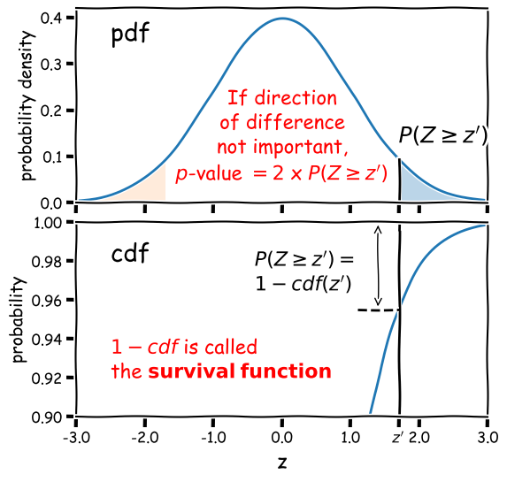
Note that the function 1-cdf is called the survival function and it is available as a separate method for the statistical distributions in
scipy.stats, which can be more accurate than calculating 1-cdf explicitly for very small \(p\)-values.For example, for the graphical example above, where the distribution is a standard normal:
print("p-value = ",2*sps.norm.sf(1.7))p-value = 0.08913092551708608In this example the significance is low and the null hypothesis is not ruled out at better than 95% confidence.
Significance levels and reporting
How should we choose our significance level, \(\alpha\)? It depends on how important is the answer to the scientific question you are asking!
- Is it a really big deal, e.g. the discovery of a new particle, or an unexpected source of emission in a given waveband (such as the first electromagnetic counterpart to a gravitational wave source)? If so, then the usual required significance is \(\alpha= 5\sigma\), which means the probability of the data being consistent with the null hypothesis (i.e. non-detection of the particle or electromagnetic counterpart) is equal or less than that in the integrated pdf more than 5 standard deviations from the mean for a standard normal distribution (\(p\simeq 5.73\times 10^{-7}\) or about 1 in 1.7 million).
- Is it important but not completely groundbreaking or requiring re-writing of or large addition to our understanding of the scientific field? For example, the ruling out of a particular part of parameter space for a candidate dark matter particle, or the discovery of emission in a known electromagnetic radiation source but in a completely different waveband to that observed before (e.g. an X-ray counterpart to an optical source)? In this case we would usually be happy with \(\alpha= 3\sigma\) (\(p\simeq 2.7\times 10^{-3}\), i.e. 0.27% probability).
- Does the analysis show (or rule out) an effect but without much consequence, since the effect (or lack of it) was already expected based on previous analysis, or as a minor consequence of well-established theory? Or is the detection of the effect tentative and only reported to guide design of future experiments or analysis of additional data? If so, then we might accept a significance level as low as \(\alpha=0.05\). This level is considered the minimum bench-mark for publication in some fields, but in physics and astronomy it is usually only considered as suitable for individual claims in a paper that also presents more significant results or novel interpretation.
When reporting results for pre-specified tests we usually state them in this way (or similar, according to your own style or that of the field):
”<The hypothesis> is rejected at the <insert \(\alpha\) here> significance level.”
‘Rule out’ is also often used as a synonym for ‘reject’. Or if we also include the calculated \(p\)-value for completeness:
“We obtained a \(p-\)value of <insert \(p\) here>”, so that the hypothesis is rejected at the <insert \(\alpha\) here> significance level.”
Sometimes we invert the numbers (taking 1 minus the \(p\)-value or probability) and report the confidence level as a percentage e.g. for \(\alpha=0.05\) we can also state:
“We rule out …. at the 95% confidence level.”
And if (as is often the case) our required significance is not satisfied, we should also state that:
“We cannot rule out …. at better than the <insert \(\alpha\) here> significance level.”
Example: comparing the sample mean with a population with known mean and variance
We’ll start with a simpler example than the speed-of-light data (where our null hypothesis only tells us the mean of the underlying population), by looking at some data where we already know both the mean and variance of the population we are comparing with.
The data consists of a sample of heights (in cm) of students in this class in previous years. The heights are given in the first column and the second column gives an integer (1 or 0) in place of the self-identified gender of the student.
From official data we have the means and standard deviations of the adult population of the Netherlands, split female/male, as follows:
- Female: \(\mu=169\) cm, \(\sigma=7.11\) cm.
- Male: \(\mu=181.1\) cm, \(\sigma=7.42\) cm.
The first question we would like to answer is, are the data from our class consistent with either (or both) of these distributions?
We’ll first load the data and split it into two subsamples according to the integer used to ID the gender. We’ll then take a look at the distribution of the two subsamples by plotting histograms. For comparison we will also plot the means of male and female heights in the Netherlands from the official data
# Load the class heights data
class_heights = np.genfromtxt("class_heights.dat")

# Create arrays of the two gender subsamples:
heights0 = class_heights[class_heights[:,1] == 0]
heights1 = class_heights[class_heights[:,1] == 1]

plt.figure()
plt.hist(heights0[:,0], bins=10, histtype='step', linewidth=4, alpha=0.5, label='subsample 0')
plt.hist(heights1[:,0], bins=10, histtype='step', linewidth=4, alpha=0.5, label='subsample 1')
plt.xlabel('height (cm)', fontsize=14)
plt.ylabel('counts', fontsize=14)
plt.axvline(181.1, label=r'$\mu_{\rm m}$', color='gray', linestyle='dashed')
plt.axvline(169, label=r'$\mu_{\rm f}$', color='gray', linestyle='dotted')
plt.legend(fontsize=12,ncol=2,columnspacing=1.0,loc=2)
plt.show()
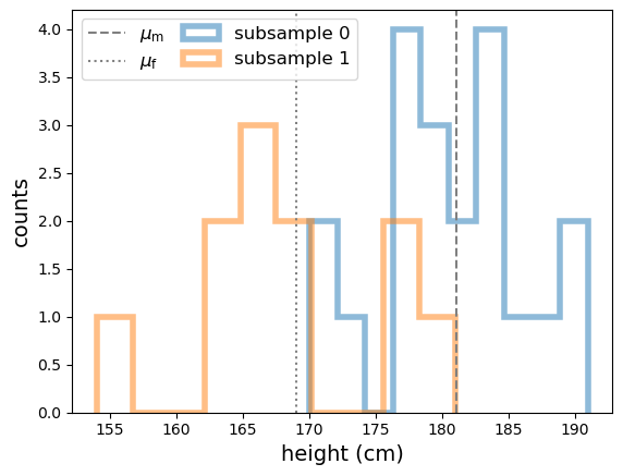
From the histograms, the two subsamples appear to be different and the difference might be explained by the difference in height distributions from the official Dutch survey data, but we need to put this on a more quantitative footing. So let’s frame our question into a testable hypothesis.
Building a testable hypothesis
To frame a scientific question into a hypothesis we can test, we need to specify two key components:
- A physical model: The component that can be described with parameters that are fixed and independent of that particular experiment.
- A statistical model: The component that leads to the specific instance of data and which may be repeated to produce a different experimental realisation of the data which is drawn from the same distribution as the previous experiment.
For example, in an experiment to measure the distribution of photon energies (i.e. a spectrum) from a synchrotron emission process, the physical model is the parameterisation of the underlying spectral shape (e.g. with a power-law index and normalisation for an empirical description) and possibly the modification of the spectrum by the instrument itself (collecting area vs. photon energy). The statistical model is that the photon detections are described by a Poisson process with rate parameter proportional to the photon flux of the underlying spectrum.
Splitting the components of the hypothesis in this way is important because it makes it easier to select an appropriate statistical test and it reminds us that a hypothesis may be rejected because the statistical model is incorrect, i.e. not necessarily because the underlying physical model is false.
Our (null) hypothesis is: A given subsample of heights is drawn from a population with mean and standard deviation given by the values for the Dutch male or female populations.
This doesn’t sound like much but now breaking it down into the statistical (red) and physical (blue) models implicit to the hypothesis:
A given subsample of class heights is drawn in an unbiased way from a population with mean and standard deviation given by the values for either of the given Dutch male or female populations.
The statistical part is subtle because parameters of the distribution are subsumed into the physical part, since these are fixed and independent of our experiment provided that the experimental sample is indeed drawn from one of these populations. Note that the statistical model of the hypothesis also covers the possibility that the subsamples are selected in different ways (gender identification is complex and also not strictly binary and we don’t know whether the quoted Dutch population statistics were based on self-identification or another method which may be biased in a different way).
Testing our hypothesis
Now we’re ready to test our hypothesis. Since we know the mean and standard deviation of our populations, the obvious statistic to test is the mean since it is an unbiased estimator. We need to make (and state!) a further assumption to continue with our test:
The sample mean is drawn from a normal distribution with mean \(\mu\) and standard deviation equal to the standard error \(\sigma/\sqrt{n}\) (where \(\mu\) and \(\sigma\) are the mean and standard deviation of the population we are comparing with and \(n\) is the number of heights in a subsample).
This assumption allows us to justify our choice of test statistic and specify the kind of test we will be using. The choice of population parameters is driven by the data, but the assumption of a normally distributed sample mean can be justified in two ways. Firstly, the assumption will hold exactly if the population height distributions are normal (this is actually the case!), since a sum (and hence mean) of normally distributed variates is itself normally distributed.
The assumption will also hold (but more weakly) if we can apply the central limit theorem to our data. Our sample sizes (\(n=20\) and \(n=11\)) are rather small for this, but it’s likely that the assumption holds for deviations at least out to 2 to 3 times \(\sigma/\sqrt{n}\) from the population means (e.g. compare with the simulations for sums of uniform variates in the previous episode).
Challenge: calculate the test statistic and its significance
Having stated our null hypothesis and assumption(s) required for the test, we now proceed with the test itself. If (as assumed) the sample means (\(\bar{x}\)) are uniformly distributed around \(\mu\) with standard deviation \(\sigma/\sqrt{n}\), we can define a new test statistic, the \(z\)-statistic
\[Z = \frac{\bar{x}-\mu}{\sigma/\sqrt{n}}\]which is distributed as a standard normal. By calculating the \(p\)-value of our statistic \(Z=z^{\prime}\) (e.g. see Significance testing: two-tailed case above) we can determine the significance of our \(z\)-test.
Now write a function that takes as input the data for a class heights subsample and the normal distribution parameters you are comparing it with, and outputs the \(p\)-value, and use your function to compare the means of each subsample with the male and female adult height distributions for the Netherlands.
Solution
def mean_significance(data,mu,sigma):
    '''Calculates the significance of a sample mean of input data vs. a specified normal distribution
    Inputs: The data (1-D array) and mean and standard deviation of normally distributed comparison population
    Outputs: prints the observed mean and population parameters, the Z statistic value and p-value'''
    mean = np.mean(data)
    # Calculate the Z statistic zmean
    zmean = np.abs((mean-mu)*np.sqrt(len(data))/sigma)
    # Calculate the p-value of zmean from the survival function - default distribution is standard normal
    pval = 2*sps.norm.sf(zmean)
    print("Observed mean =",mean," versus population mean",mu,", sigma",sigma)
    print("z_mean =",zmean,"with Significance =",pval)
    return
Now running the function with the data and given population parameters:
print("\nComparing with Dutch female height distribution:")
mu, sigma = 169, 7.11
print("\nSubsample 0:")
mean_significance(heights0[:,0],mu,sigma)
print("\nSubsample 1:")
mean_significance(heights1[:,0],mu,sigma)

print("\nComparing with Dutch male height distribution:")
mu, sigma = 181.1, 7.42
print("\nSubsample 0:")
mean_significance(heights0[:,0],mu,sigma)
print("\nSubsample 1:")
mean_significance(heights1[:,0],mu,sigma)
Comparing with Dutch female height distribution: Subsample 0: Observed mean = 180.6 versus population mean 169 , sigma 7.11 z_mean = 1.6315049226441622 with Significance = 0.10278382199989615 Subsample 1: Observed mean = 168.0909090909091 versus population mean 169 , sigma 7.11 z_mean = 0.12786088735455786 with Significance = 0.8982590642895918 Comparing with Dutch male height distribution: Subsample 0: Observed mean = 180.6 versus population mean 181.1 , sigma 7.42 z_mean = 0.0673854447439353 with Significance = 0.9462748562617406 Subsample 1: Observed mean = 168.0909090909091 versus population mean 181.1 , sigma 7.42 z_mean = 1.7532467532467522 with Significance = 0.07955966096511223
We can see that the means of both subsamples are formally consistent with being drawn from either population, although the significance for subsample 0 is more consistent with the male population than the female, and vice versa for subsample 1. Formally we can state that none of the hypotheses are ruled out at more than 95% confidence.
Our results seem inconclusive in this case, however here we have only performed significance tests of each hypothesis individually. We can also ask a different question, which is: is one hypothesis (i.e. in this case one population) preferred over another at a given confidence level? We will cover this form of hypothesis comparison in a later episode.
Key Points
Significance testing is used to determine whether a given (null) hypothesis is rejected by the data, by calculating a test statistic and comparing it with the distribution expected for it, under the assumption that the null hypothesis is true.
A null hypothesis is formulated from a physical model (with parameters that are fixed and independent of the experiment) and a statistical model (which governs the probability distribution of the test statistic). Additional assumptions may be required to derive the distribution of the test statistic.
A null hypothesis is rejected if the measured p-value of the test statistic is equal to or less than a pre-defined significance level.
Rejection of the null hypothesis could indicate rejection of either the physical model or the statistical model (or both), with further experiments or tests required to determine which.
For comparing measurements with an expected (population mean) value, a z-statistic can be calculated to compare the sample mean with the expected value, normalising by the standard error on the sample mean, which requires knowledge of the variance of the population that the measurements are sampled from.
The z-statistic should be distributed as a standard normal provided that the sample mean is normally distributed, which may arise for large samples from the central limit theorem, or for any sample size if the measurements are drawn from normal distributions.