Discrete random variables and their probability distributions

Overview

Teaching: 40 min
Exercises: 10 min

Questions

• How do we describe discrete random variables and what are their common probability distributions?

Objectives

• Learn how discrete random variables are defined and how the Bernoulli, binomial and Poisson distributions are derived from them.

• Plot, and carry out probability calculations with the binomial and Poisson distributions.

In this episode we will be using numpy, as well as matplotlib’s plotting library. Scipy contains an extensive range of distributions in its ‘scipy.stats’ module, so we will also need to import it. Remember: scipy modules should be installed separately as required - they cannot be called if only scipy is imported.

import numpy as np
import matplotlib.pyplot as plt
import scipy.stats as sps

So far we have only considered random variables that are drawn from continuous distributions, such as the important uniform and normal distributions. However, random variables can also be discrete, drawn from (finite or infinite) sets of discrete values and including some of the most important probability distributions in statistics, such as the binomial and Poisson distributions. We will spend some time considering discrete random variables and their distributions here.

Sample space

Discrete probability distributions map a sample space \(\Omega\) (denoted with curly brackets) of possible outcomes on to a set of corresponding probabilities. Unlike continuous distributions, the sample space may consist of non-numerical elements or numerical elements, but in all cases the elements of the sample space represent possible outcomes of a random ‘draw’ from the distribution.

For example, when flipping an ideal coin (which cannot land on its edge!) there are two outcomes, heads (\(H\)) or tails (\(T\)) so we have the sample space \(\Omega = \{H, T\}\). We can also represent the possible outcomes of 2 successive coin flips as the sample space \(\Omega = \{HH, HT, TH, TT\}\). A roll of a 6-sided dice would give \(\Omega = \{1, 2, 3, 4, 5, 6\}\). However, a Poisson process corresponds to the sample space \(\Omega = \mathbb{Z}^{0+}\), i.e. the set of all positive and integers and zero, even if the probability for most elements of that sample space is infinitesimal (it is still \(> 0\)!).

Probability distributions of discrete random variables

In the case of a Poisson process or the roll of a dice, our sample space already consists of a set of contiguous (i.e. next to one another in sequence) numbers which correspond to discrete random variables. Where the sample space is categorical, such as heads or tails on a coin, or perhaps a set of discrete but non-integer values (e.g. a pre-defined set of measurements to be randomly drawn from), it is useful to map the elements of the sample space on to a set of integers which then become our discrete random variables \(X\). For example, when flipping a coin, define a variable \(X\):

We can write the probability that \(X\) has a value \(x\) as \(p(x) = P(X=x)\), so that assuming the coin is fair, we have \(p(0) = p(1) = 0.5\). Our definition therefore allows us to map discrete but non-integer outcomes on to numerically ordered integer random variables \(X\) for which we can construct a probability distribution. Using this approach we can define the cdf for discrete random variables as:

where the subscript \(i\) corresponds to the numerical ordering of a given outcome, i.e. of an element in the sample space. The survival function is equal to \(P(X\gt x)\).

It should be clear that for discrete random variables there is no direct equivalent of the pdf for probability distributions of discrete random variables, but the function \(p(x)\) is generally specified for a given distribution instead and is known as the probability mass function or pmf.

Random sampling of items in a list or array

If you want to simulate random sampling of elements in a sample space, a simple way to do this is to set up a list or array containing the elements and then use the numpy function numpy.random.choice to select from the list. As a default, sampling probabilities are assumed to be \(1/n\) for a list with \(n\) items, but they may be set using the p argument to give an array of p-values for each element in the sample space. The replace argument sets whether the sampling should be done with or without replacement.

For example, to set up 10 repeated flips of a coin, for an unbiased and a biased coin:

coin = ['h','t']
# Uses the defaults (uniform probability, replacement=True)
print("Unbiased coin: ",np.random.choice(coin, size=10))
# Now specify probabilities to strongly weight towards heads:
prob = [0.9,0.1]
print("Biased coin: ",np.random.choice(coin, size=10, p=prob))

Unbiased coin:  ['h' 'h' 't' 'h' 'h' 't' 'h' 't' 't' 'h']
Biased coin:  ['h' 'h' 't' 'h' 'h' 't' 'h' 'h' 'h' 'h']

Properties of discrete random variables

Similar to the calculations for continuous random variables, expectation values of discrete random variables (or functions of them) are given by the probability-weighted values of the variables or their functions:

Probability distributions: Bernoulli and Binomial

A Bernoulli trial is a draw from a sample with only two possibilities (e.g. the colour of sweets drawn, with replacement, from a bag of red and green sweets). The outcomes are mapped on to integer variates \(X=1\) or \(0\), assuming probability of one of the outcomes \(\theta\), so the probability \(p(x)=P(X=x)\) is:

and the corresponding Bernoulli distribution function (the pmf) can be written as:

A variate drawn from this distribution is denoted as \(X\sim \mathrm{Bern}(\theta)\) and has \(E[X]=\theta\) and \(V[X]=\theta(1-\theta)\) (which can be calculated using the equations for discrete random variables above).

We can go on to consider what happens if we have repeated Bernoulli trials. For example, if we draw sweets with replacement (i.e. we put the drawn sweet back before drawing again, so as not to change \(\theta\)), and denote a ‘success’ (with \(X=1\)) as drawing a red sweet, we expect the probability of drawing \(red, red, green\) (in that order) to be \(\theta^{2}(1-\theta)\).

However, what if we don’t care about the order and would just like to know the probability of getting a certain number of successes from \(n\) draws or trials (since we count each draw as a sampling of a single variate)? The resulting distribution for the number of successes (\(x\)) as a function of \(n\) and \(\theta\) is called the binomial distribution:

Note that the matrix term in brackets is the binomial coefficient to account for the permutations of the ordering of the \(x\) successes. For variates distributed as \(X\sim \mathrm{Binom}(n,\theta)\), we have \(E[X]=n\theta\) and \(V[X]=n\theta(1-\theta)\).

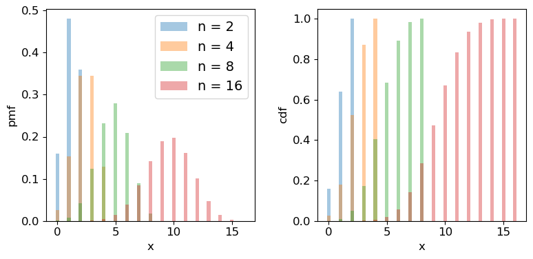
Naturally, scipy has a binomial distribution in its stats module, with the usual functionality, although note that the pmf method replaces the pdf method for discrete distributions. Below we plot the pmf and cdf of the distribution for different numbers of trials \(n\). It is formally correct to plot discrete distributions using separated bars, to indicate single discrete values, rather than bins over multiple or continuous values, but sometimes stepped line plots (or even histograms) can be clearer, provided you explain what they show.

## Define theta
theta = 0.6
## Plot as a bar plot
fig, (ax1, ax2) = plt.subplots(1,2, figsize=(9,4))
fig.subplots_adjust(wspace=0.3)
for n in [2,4,8,16]:
    x = np.arange(0,n+1)
    ## Plot the pmf
    ax1.bar(x, sps.binom.pmf(x,n,p=theta), width=0.3, alpha=0.4, label='n = '+str(n))
    ## and the cumulative distribution function:
    ax2.bar(x, sps.binom.cdf(x,n,p=theta), width=0.3, alpha=0.4, label='n = '+str(n))
for ax in (ax1,ax2):
    ax.tick_params(labelsize=12)
    ax.set_xlabel("x", fontsize=12)
    ax.tick_params(axis='x', labelsize=12)
    ax.tick_params(axis='y', labelsize=12)
ax1.set_ylabel("pmf", fontsize=12)
ax2.set_ylabel("cdf", fontsize=12)
ax1.legend(fontsize=14)
plt.show()

Challenge: how many observations do I need?

Imagine that you are developing a research project to study the radio-emitting counterparts of binary neutron star mergers that are detected by a gravitational wave detector. Due to relativistic beaming effects however, radio counterparts are not always detectable (they may be beamed away from us). You know from previous observations and theory that the probability of detecting a radio counterpart from a binary neutron star merger detected by gravitational waves is 0.72. For simplicity you can assume that you know from the gravitational wave signal whether the merger is a binary neutron star system or not, with no false positives.

You need to request a set of observations in advance from a sensitive radio telescope to try to detect the counterparts for each binary merger detected in gravitational waves. You need 10 successful detections of radio emission in different mergers, in order to test a hypothesis about the origin of the radio emission. Observing time is expensive however, so you need to minimise the number of observations of different binary neutron star mergers requested, while maintaining a good chance of success. What is the minimum number of observations of different mergers that you need to request, in order to have a better than 95% chance of being able to test your hypothesis?

(Note: all the numbers here are hypothetical, and are intended just to make an interesting problem!)

Solution

We want to know the number of trials \(n\) for which we have a 95% probability of getting at least 10 detections. Remember that the cdf is defined as \(F(x) = P(X\leq x)\), so we need to use the survival function (1-cdf) but for \(x=9\), so that we calculate what we need, which is \(P(X\geq 10)\). We also need to step over increasing values of \(n\) to find the smallest value for which our survival function exceeds 0.95. We will look at the range \(n=\)10-25 (there is no point in going below 10!).

theta = 0.72
for n in range(10,26):
    print("For",n,"observations, chance of 10 or more detections =",sps.binom.sf(9,n,p=theta))

For 10 observations, chance of 10 or more detections = 0.03743906242624486
For 11 observations, chance of 10 or more detections = 0.14226843721973037
For 12 observations, chance of 10 or more detections = 0.3037056744016985
For 13 observations, chance of 10 or more detections = 0.48451538004550243
For 14 observations, chance of 10 or more detections = 0.649052212181364
For 15 observations, chance of 10 or more detections = 0.7780490885758796
For 16 observations, chance of 10 or more detections = 0.8683469020520406
For 17 observations, chance of 10 or more detections = 0.9261375026767835
For 18 observations, chance of 10 or more detections = 0.9605229100485057
For 19 observations, chance of 10 or more detections = 0.9797787381766699
For 20 observations, chance of 10 or more detections = 0.9900228387408534
For 21 observations, chance of 10 or more detections = 0.9952380172098922
For 22 observations, chance of 10 or more detections = 0.9977934546597212
For 23 observations, chance of 10 or more detections = 0.9990043388667172
For 24 observations, chance of 10 or more detections = 0.9995613456019353
For 25 observations, chance of 10 or more detections = 0.999810884619313

So we conclude that we need 18 observations of different binary neutron star mergers, to get a better than 95% chance of obtaining 10 radio detections.

Probability distributions: Poisson

Imagine that we are running a particle detection experiment, e.g. to detect radioactive decays. The particles are detected with a fixed mean rate per time interval \(\lambda\). To work out the distribution of the number of particles \(x\) detected in the time interval, we can imagine splitting the interval into \(n\) equal sub-intervals. Then, if the mean rate \(\lambda\) is constant and the detections are independent of one another, the probability of a detection in any given time interval is the same: \(\lambda/n\). We can think of the sub-intervals as a set of \(n\) repeated Bernoulli trials, so that the number of particles detected in the overall time-interval follows a binomial distribution with \(\theta = \lambda/n\):

In reality the distribution of possible arrival times in an interval is continuous and so we should make the sub-intervals infinitesimally small, otherwise the number of possible detections would be artificially limited to the finite and arbitrary number of sub-intervals. If we take the limit \(n\rightarrow \infty\) we obtain the follow useful results:

\(\frac{n!}{(n-x)!} = \prod\limits_{i=0}^{x-1} (n-i) \rightarrow n^{x}\) and \(\lim\limits_{n\rightarrow \infty} (1-\lambda/n)^{n-x} = e^{-\lambda}\)

where the second limit arises from the result that \(e^{x} = \lim\limits_{n\rightarrow \infty} (1+x/n)^{n}\). Substituting these terms into the expression from the binomial distribution we obtain:

This is the Poisson distribution, one of the most important distributions in observational science, because it describes counting statistics, i.e. the distribution of the numbers of counts in bins. For example, although we formally derived it here as being the distribution of the number of counts in a fixed interval with mean rate \(\lambda\) (known as a rate parameter), the interval can refer to any kind of binning of counts where individual counts are independent and \(\lambda\) gives the expected number of counts in the bin.

For a random variate distributed as a Poisson distribution, \(X\sim \mathrm{Pois}(\lambda)\), \(E[X] = \lambda\) and \(V[X] = \lambda\). The expected variance leads to the expression that the standard deviation of the counts in a bin is equal to \(\sqrt{\lambda}\), i.e. the square root of the expected value. We will see later on that for a Poisson distributed likelihood, the observed number of counts is an estimator for the expected value. From this, we obtain the famous \(\sqrt{counts}\) error due to counting statistics.

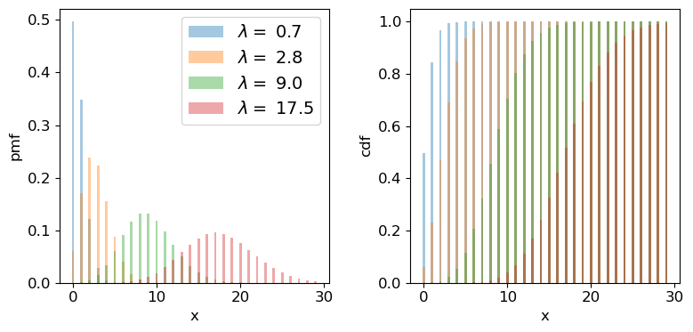
We can plot the Poisson pmf and cdf in a similar way to how we plotted the binomial distribution functions. An important point to bear in mind is that the rate parameter \(\lambda\) does not itself have to be an integer: the underlying rate is likely to be real-valued, but the Poisson distribution produces integer variates drawn from the distribution that is unique to \(\lambda\).

## Plot as a bar plot
fig, (ax1, ax2) = plt.subplots(1,2, figsize=(9,4))
fig.subplots_adjust(wspace=0.3)
## Step through lambda, note that to avoid Python confusion with lambda functions, we make sure we choose
## a different variable name!
for lam in [0.7,2.8,9.0,17.5]:
    x = np.arange(0,30)
    ## Plot the pmf, note that perhaps confusingly, the rate parameter is defined as mu
    ax1.bar(x, sps.poisson.pmf(x,mu=lam), width=0.3, alpha=0.4, label='$\lambda =$ '+str(lam))
    ## and the cumulative distribution function:
    ax2.bar(x, sps.poisson.cdf(x,mu=lam), width=0.3, alpha=0.4, label='$\lambda =$ '+str(lam))
for ax in (ax1,ax2):
    ax.tick_params(labelsize=12)
    ax.set_xlabel("x", fontsize=12)
    ax.tick_params(axis='x', labelsize=12)
    ax.tick_params(axis='y', labelsize=12)
ax1.set_ylabel("pmf", fontsize=12)
ax2.set_ylabel("cdf", fontsize=12)
ax1.legend(fontsize=14)
plt.show()

Challenge: how long until the data are complete?

Following your successful proposal for observing time, you’ve been awarded 18 radio observations of neutron star binary mergers (detected via gravitational wave emission) in order to search for radio emitting counterparts. The expected detection rate for gravitational wave events from binary neutron star mergers is 9.5 per year. Assume that you require all 18 observations to complete your proposed research. You will need to resubmit your proposal if it isn’t completed within 3 years. What is the probability that you will need to resubmit your proposal?

Solution

Since binary mergers are independent random events and their mean detection rate (at least for a fixed detector sensitivity and on the time-scale of the experiment!) should be constant in time, the number of merger events in a fixed time interval should follow a Poisson distribution.

Given that we require the full 18 observations, the proposal will need to be resubmitted if there are fewer than 18 gravitational wave events (from binary neutron stars) in 3 years. For this we can use the cdf, remember again that for the cdf \(F(x) = P(X\leq x)\), so we need the cdf for 17 events. The interval we are considering is 3 years not 1 year, so we should multiply the annual detection rate by 3 to get the correct \(\lambda\):

lam = 9.5*3
print("Probability that < 18 observations have been carried out in 3 years =",sps.poisson.cdf(17,lam))

Probability that < 18 observations have been carried out in 3 years = 0.014388006538141204

So there is only a 1.4% chance that we will need to resubmit our proposal.

Challenge: is this a significant detection?

Meanwhile, one of your colleagues is part of a team using a sensitive neutrino detector to search for bursts of neutrinos associated with neutron star mergers detected from gravitational wave events. The detector has a constant background rate of 0.03 count/s. In a 1 s window following a gravitational wave event, the detector detects a single neutrino. Calculate the \(p\)-value of this detection, for the null hypothesis that it is just produced by the background and state the corresponding significance level in \(\sigma\). What would the significance levels be (in \(\sigma\)) for 2, and 3 detected neutrinos?

Discrete random variables and the central limit theorem

Finally, we should bear in mind that, as with other distributions, in the large sample limit the binomial and Poisson distributions both approach the normal distribution, with mean and standard deviation given by the expected values for the discrete distributions (i.e. \(\mu=n\theta\) and \(\sigma=\sqrt{n\theta(1-\theta)}\) for the binomial distribution and \(\mu = \lambda\) and \(\sigma = \sqrt{\lambda}\) for the Poisson distribution). It’s easy to do a simple comparison yourself, by overplotting the Poisson or binomial pdfs on those for the normal distribution.

Key Points

• Discrete probability distributions map a sample space of discrete outcomes (categorical or numerical) on to their probabilities.

• By assigning an outcome to an ordered sequence of integers corresponding to the discrete variates, functional forms for probability distributions (the pmf or probability mass function) can be defined.

• Bernoulli trials correspond to a single binary outcome (success/fail) while the number of successes in repeated Bernoulli trials is given by the binomial distribution.

• The Poisson distribution can be derived as a limiting case of the binomial distribution and corresponds to the probability of obtaining a certain number of counts in a fixed interval, from a random process with a constant rate.

• Counts in fixed histogram bins follow Poisson statistics.

• In the limit of large numbers of successes/counts, the binomial and Poisson distributions approach the normal distribution.