Bayes' Theorem

Overview

Teaching: 30 min
Exercises: 30 min

Questions

• What is Bayes’ theorem and how can we use it to answer scientific questions?

Objectives

• Learn how Bayes’ theorem is derived and how it applies to simple probability problems.

• Learn how to derive posterior probability distributions for simple hypotheses, both analytically and using a Monte Carlo approach.

In this episode we will be using numpy, as well as matplotlib’s plotting library. Scipy contains an extensive range of distributions in its ‘scipy.stats’ module, so we will also need to import it. Remember: scipy modules should be installed separately as required - they cannot be called if only scipy is imported.

import numpy as np
import matplotlib.pyplot as plt
import scipy.stats as sps

When considering two events \(A\) and \(B\), we have previously seen how the equation for conditional probability gives us the multiplication rule:

It should be clear that we can invert the ordering of \(A\) and \(B\) here and the probability of both happening should still be the same, i.e.:

This simple extension of probability calculus leads us to Bayes’ theorem, one of the most important results in statistics and probability theory:

Bayes’ theorem, named after clergyman Rev. Thomas Bayes who proposed it in the middle of the 18th century, is in its simplest form, a method to swap the conditional dependence of two events, i.e. to obtain the probability of \(A\) conditional on \(B\), when you only know the probability of \(B\) conditional on \(A\), and the probabilities of \(A\) and \(B\) (i.e. each marginalised over the conditional term).

To show the inclusion of marginalisation, we can generalise from two events to a set of mutually exclusive exhaustive events \(\{A_{1},A_{2},...,A_{n}\}\):

Challenge: what kind of binary merger is it?

Returning to our hypothetical problem of detecting radio counterparts from gravitational wave events corresponding to binary mergers of binary neutron stars (NN), binary black holes (BB) and neutron star-black hole binaries (NB), recall that the probabilities of radio detection (event denoted with \(D\)) are:

\(P(D\vert NN) = 0.72\), \(P(D\vert NB) = 0.2\), \(P(D\vert BB) = 0\)

and for any given merger event the probability of being a particular type of binary is:

\(P(NN)=0.05\), \(P(NB) = 0.2\), \(P(BB)=0.75\)

Calculate the following:

1. Assuming that you detect a radio counterpart, what is the probability that the event is a binary neutron star (\(NN\))?
2. Assuming that you \(don't\) detect a radio counterpart, what is the probability that the merger includes a black hole (either \(BB\) or \(NB\))?

Hint

Remember that if you need a total probability for an event for which you only have the conditional probabilities, you can use the law of total probability and marginalise over the conditional terms.

Solution

1. We require \(P(NN\vert D)\). Using Bayes’ theorem: \(P(NN\vert D) = \frac{P(D\vert NN)P(NN)}{P(D)}\) We must marginalise over the conditionals to obtain \(P(D)\), so that:

   \(P(NN\vert D) = \frac{P(D\vert NN)P(NN)}{(P(D\vert NN)P(NN)+P(D\vert NB)P(NB)} = \frac{0.72\times 0.05}{(0.72\times 0.05)+(0.2\times 0.2)}\) \(= \frac{0.036}{0.076} = 0.474 \mbox{ (to 3 s.f.)}\)

2. We require \(P(BB \vert D^{C}) + P(NB \vert D^{C})\), since radio non-detection is the complement of \(D\) and the \(BB\) and \(NB\) events are mutually exclusive. Therefore, using Bayes’ theorem we should calculate:

   \[P(BB \vert D^{C}) = \frac{P(D^{C} \vert BB)P(BB)}{P(D^{C})} = \frac{1\times 0.75}{0.924} = 0.81169\] \[P(NB \vert D^{C}) = \frac{P(D^{C} \vert NB)P(NB)}{P(D^{C})} = \frac{0.8\times 0.2}{0.924} = 0.17316\]

So our final result is: \(P(BB \vert D^{C}) + P(NB \vert D^{C}) = 0.985 \mbox{ (to 3 s.f.)}\)

Here we used the fact that \(P(D^{C})=1-P(D)\), along with the value of \(P(D)\) that we already calculated in part 1.

There are a few interesting points to note about the calculations:

• Firstly, in the absence of any information from the radio data, our prior expectation was that a merger would most likely be a black hole binary (with 75% chance). As soon as we obtained a radio detection, this chance went down to zero.
• Then, although the prior expectation that the merger would be of a binary neutron star system was 4 times smaller than that for a neutron star-black hole binary, the fact that a binary neutron star was almost 4 times more likely to be detected in radio almost balanced the difference, so that we had a slightly less than 50/50 chance that the system would be a binary neutron star.
• Finally, it’s worth noting that the non-detection case weighted the probability that the source would be a black hole binary to slightly more than the prior expectation of \(P(BB)=0.75\), and correspondingly reduced the expectation that the system would be a neutron star-black hole system, because there is a moderate chance that such a system would produce radio emission, which we did not see.

Bayes’ theorem for continuous probability distributions

From the multiplication rule for continuous probability distributions, we can obtain the continuous equivalent of Bayes’ theorem:

Bayes’ billiards game

This problem is taken from the useful article Frequentism and Bayesianism: A Python-driven Primer by Jake VanderPlas, and is there adapted from a problem discussed by Sean J. Eddy.

Carol rolls a billiard ball down the table, marking where it stops. Then she starts rolling balls down the table. If the ball lands to the left of the mark, Alice gets a point, to the right and Bob gets a point. First to 6 points wins. After some time, Alice has 5 points and Bob has 3. What is the probability that Bob wins the game (\(P(B)\))?

Defining a success as a roll for Alice (so that she scores a point) and assuming the probability \(p\) of success does not change with each roll, the relevant distribution is binomial. For Bob to win, he needs the next three rolls to fail (i.e. the points go to him). A simple approach is to estimate \(p\) using the number of rolls and successes, since the expectation for \(X\sim \mathrm{Binom}(n,p)\) is \(E[X]=np\), so taking the number of successes as an unbiased estimator, our estimate for \(p\), \(\hat{p}=5/8\). Then the probability of failing for three successive rolls is:

\[(1-\hat{p})^{3} \simeq 0.053\]

However, this approach does not take into account our uncertainty about Alice’s true success rate!

Let’s use Bayes’ theorem. We want the probability that Bob wins given the data already in hand (\(D\)), i.e. the \((5,3)\) scoring. We don’t know the value of \(p\), so we need to consider the marginal probability of \(B\) with respect to \(p\):

\[P(B\vert D) \equiv \int P(B,p \vert D) \mathrm{d}p\]

We can use the multiplication rule \(P(A \mbox{ and } B) = P(A\vert B) P(B)\), since \(P(B,p \vert D) \equiv P(B \mbox{ and } p \vert D)\):

\[P(B\vert D) = \int P(B\vert p, D) P(p\vert D) \mathrm{d}p\]

Now we can calculate \(P(D\vert p)\) from the binomial distribution, so to get there we use Bayes’ theorem:

\[P(B\vert D) = \int P(B\vert p, D) \frac{P(D\vert p)P(p)}{P(D)} \mathrm{d}p\] \[= \frac{\int P(B\vert p, D) P(D\vert p)P(p) \mathrm{d}p}{\int P(D\vert p)P(p)\mathrm{d}p}\]

where we first take \(P(D)\) outside the integral (since it has no explicit \(p\) dependence) and then express it as the marginal probability over \(p\). Now:

• The term \(P(B\vert p,D)\) is just the binomial probability of 3 failures for a given \(p\), i.e. \(P(B\vert p,D) = (1-p)^{3}\) (conditionality on \(D\) is implicit, since we know the number of consecutive failures required).
• \(P(D\vert p)\) is just the binomial probability from 5 successes and 3 failures, \(P(D\vert p) \propto p^{5}(1-p)^{3}\). We ignore the term accounting for permutations and combinations since it is constant for a fixed number of trials and successes, and cancels from the numerator and denominator.
• Finally we need to consider the distribution of the chance of a success, \(P(p)\). This is presumably based on Carol’s initial roll and success rate, which we have no prior expectation of, so the simplest assumption is to assume a uniform distribution (i.e. a uniform prior): \(P(p)= constant\), which also cancels from the numerator and denominator.

Finally, we solve:

\[P(B\vert D) = \frac{\int_{0}^{1} (1-p)^{6}p^{5}}{\int_{0}^{1} (1-p)^{3}p^{5}} \simeq 0.091\]

The probability of success for Bob is still low, but has increased compared to our initial, simple estimate. The reason for this is that our choice of prior suggests the possibility that \(\hat{p}\) overestimated the success rate for Alice, since the median \(\hat{p}\) suggested by the prior is 0.5, which weights the success rate for Alice down, increasing the chances for Bob.

Bayes’ Anatomy

Consider a hypothesis \(H\) that we want to test with some data \(D\). The hypothesis may, for example be about the true value of a model parameter or its distribution.

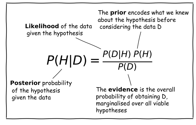
Scientific questions usually revolve around whether we should favour a particular hypothesis, given the data we have in hand. In probabilistic terms we want to know \(P(H\vert D)\), which is known as the posterior probability or sometimes just ‘the posterior’.

However, you have already seen that the statistical tests we can apply to assess probability work the other way around. We know how to calculate how likely a particular set of data is to occur (e.g. using a test statistic), given a particular hypothesis (e.g. the value of a population mean) and associated assumptions (e.g. that the data are normally distributed).

Therefore we usually know \(P(D\vert H)\), a term which is called the likelihood since it refers to the likelihood of obtaining the data (or some statistic calculated from it), given our hypothesis. Note that there is a subtle but important difference between the likelihood and the pdf. The pdf gives the probability distribution of the variate(s) (the data or test statistic) for a given hypothesis and its (fixed) parameters. The likelihood gives the probability for fixed variate(s) as a function of the hypothesis parameters.

We also need the prior probability or just ‘the prior’, \(P(H)\) which represents our prior knowledge or belief about whether the given hypothesis is likely or not, or what we consider plausible parameter values. The prior is one of the most famous aspects of Bayes’ theorem and explicit use of prior probabilities is a key difference between Bayesian or Frequentist approaches to statistics.

Finally, we need to normalise our prior-weighted likelihood by the so-called evidence, \(P(D)\), a term corresponding to the probability of obtaining the given data, regardless of the hypothesis or its parameters. This term can be calculated by marginalising over the possible parameter values and (in principle) whatever viable, alternate hypotheses can account for the data. In practice, unless the situation is simple or very well constrained, this term is the hardest to calculate. For this reason, many calculations of the posterior probability make use of Monte Carlo methods (i.e. simulations with random variates), or assume simplifications that allow \(P(D)\) to be simplified or cancelled in some way (e.g. uniform priors). The evidence is the same for different hypotheses that explain the same data, so it can also be ignored when comparing the relative probabilities of different hypotheses.

Challenge: what is the true GW event rate?

In 1 year of monitoring with a hypothetical gravitational wave (GW) detector, you observe 4 GW events from binary neutron stars. Based on this information, you want to calculate the probability distribution of the annual rate of detectable binary neutron star mergers \(\lambda\).

From the Poisson distribution, you can write down the equation for the probability that you detect 4 GW in 1 year given a value for \(\lambda\). Use this equation with Bayes’ theorem to write an equation for the posterior probability distribution of \(\lambda\) given the observed rate, \(x\) and assuming a prior distribution for \(\lambda\), \(p(\lambda)\). Then, assuming that the prior distribution is uniform over the interval \([0,\infty]\) (since the rate cannot be negative), derive the posterior probability distribution for the observed \(x=4\). Calculate the expectation for your distribution (i.e. the distribution mean).

Hint

You will find this function useful for generating the indefinite integrals you need: \(\int x^{n} e^{-x}\mathrm{d}x = -e^{-x}\left(\sum\limits_{k=0}^{n} \frac{n!}{k!} x^{k}\right) + \mathrm{constant}\)

Solution

The posterior probability is \(p(\lambda \vert x)\) - we know \(p(x \vert \lambda)\) (the Poisson distribution, in this case) and we assume a prior \(p(\lambda)\), so we can write down Bayes’ theorem to find \(p(\lambda \vert x)\) as follows:
\(p(\lambda \vert x) = \frac{p(x \vert \lambda) p(\lambda)}{p(x)} = \frac{p(x \vert \lambda) p(\lambda)}{\int_{0}^{\infty} p(x \vert \lambda) p(\lambda) \mathrm{d}\lambda}\)

Where we use the law of total probability we can write \(p(x)\) in terms of the conditional probability and prior (i.e. we integrate the numerator in the equation). For a uniform prior, \(p(\lambda)\) is a constant, so it can be taken out of the integral and cancels from the top and bottom of the equation: \(p(\lambda \vert x) = \frac{p(x \vert \lambda)}{\int_{0}^{\infty} p(x \vert \lambda)\mathrm{d}\lambda}\)

From the Poisson distribution \(p(x \vert \lambda) = \lambda^{x} \frac{e^{-\lambda}}{x!}\), so for \(x=4\) we have \(p(x \vert \lambda) = \lambda^{4} \frac{e^{-\lambda}}{4!}\). We usually use the Poisson distribution to calculate the pmf for variable integer counts \(x\) (this is also forced on us by the function’s use of the factorial of \(x\)) and fixed \(\lambda\). But here we are fixing \(x\) and looking at the dependence of \(p(x\vert \lambda)\) on \(\lambda\), which is a continuous function. In this form, where we fix the random variable, i.e. the data (the value of \(x\) in this case) and consider instead the distribution parameter(s) as the variable, the distribution is known as a likelihood function.

So we now have:
\(p(\lambda \vert x) = \frac{\lambda^{4} \exp(-\lambda)/4!}{\int_{0}^{\infty} \left(\lambda^{4} \exp(-\lambda)/4!\right) \mathrm{d}\lambda} = \lambda^{4} \exp(-\lambda)/4!\)

since (e.g. using the hint above), \(\int_{0}^{\infty} \left(\lambda^{4} \exp(-\lambda)/4!\right) \mathrm{d}\lambda=4!/4!=1\). This latter result is not surprising, because it corresponds to the integrated probability over all possible values of \(\lambda\), but bear in mind that we can only integrate over the likelihood because we were able to divide out the prior probability distribution.

The mean is given by \(\int_{0}^{\infty} \left(\lambda^{5} \exp(-\lambda)/4!\right) \mathrm{d}\lambda = 5!/4! =5\).

Intuition builder: simulating the true event rate distribution

Now we have seen how to calculate the posterior probability for \(\lambda\) analytically, let’s see how this can be done computationally via the use of scipy’s random number generators. Such an approach is known as a Monte Carlo integration of the posterior probability distribution. Besides obtaining the mean, we can also use this approach to obtain the confidence interval on the distribution, that is the range of values of \(\lambda\) which contain a given amount of the probability. The method is also generally applicable to different, non-uniform priors, for which the analytic calculation approach may not be straightforward, or even possible.

The starting point here is the equation for posterior probability:

\[p(\lambda \vert x) = \frac{p(x \vert \lambda) p(\lambda)}{p(x)}\]

The right hand side contains two probability distributions. By generating random variates from these distributions, we can simulate the posterior distribution simply by counting the values which satisfy our data, i.e. for which \(x=4\). Here is the procedure:

1. Simulate a large number (\(\geq 10^{6}\)) of possible values of \(\lambda\), by drawing them from the uniform prior distribution. You don’t need to extend the distribution to \(\infty\), just to large enough \(\lambda\) that the observed \(x=4\) becomes extremely unlikely. You should simulate them quickly by generating one large numpy array using the size argument of the rvs method for the scipy.stats distribution.
2. Now use your sample of draws from the prior as input to generate the same number of draws from the scipy.stats Poisson probability distribution. I.e. use your array of \(\lambda\) values drawn from the prior as the input to the argument mu, and be sure to set size to be equal to the size of your array of \(\lambda\). This will generate a single Poisson variate for each draw of \(\lambda\).
3. Now make a new array, selecting only the elements from the \(\lambda\) array for which the corresponding Poisson variate is equal to 4 (our observed value).
4. The histogram of the new array of \(\lambda\) values follows the posterior probability distribution for \(\lambda\). The normalising ‘evidence’ term \(p(x)\) is automatically accounted for by plotting the histogram as a density distribution (so the histogram is normalised by the number of \(x=4\) values). You can also use this array to calculate the mean of the distribution and other statistical quantities, e.g. the standard deviation and the 95% confidence interval (which is centred on the median and contains 0.95 total probability).

Now carry out this procedure to obtain a histogram of the posterior probability distribution for \(\lambda\), the mean of this distribution and the 95% confidence interval.

Solution

# Set the number of draws to be very large
ntrials = 10000000  
# Set the upper boundary of the uniform prior (lower boundary is zero)
uniform_upper = 20
# Now draw our set of lambda values from the prior
lam_draws = sps.uniform.rvs(loc=0,scale=uniform_upper,size=ntrials)

# And use as input to generate Poisson variates each drawn from a distribution with
# one of the drawn lambda values:
poissvars = sps.poisson.rvs(mu=lam_draws, size=ntrials)

## Plot the distribution of Poisson variates drawn for the prior-distributed lambdas
plt.figure()
# These are integers, so use bins in steps of 1 or it may look strange
plt.hist(poissvars,bins=np.arange(0,2*uniform_upper,1.0),density=True,histtype='step')
plt.xlabel('$x$',fontsize=14)
plt.ylabel('Probability density',fontsize=14)
plt.show()

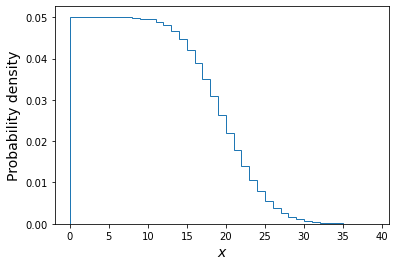
The above plot shows the distribution of the \(x\) values each corresponding to one draw of a Poisson variate with rate \(\lambda\) drawn from a uniform distribution \(U(0,20)\). Of these we will only choose those with \(x=4\) and plot their \(\lambda\) distribution below.

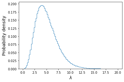
plt.figure()
## Here we use the condition poissvars==4 to select only values of lambda which 
## generated the observed value of x. Then we plot the resulting distribution
plt.hist(lam_draws[poissvars==4],bins=100, density=True,histtype='step')
plt.xlabel('$\lambda$',fontsize=14)
plt.ylabel('Probability density',fontsize=14)
plt.show()

We also calculate the mean, standard deviation and the median and 95% confidence interval around it:

print("Mean of lambda = ",np.mean(lam_draws[poissvars==4]))
print("Standard deviation of lambda = ",np.std(lam_draws[poissvars==4],ddof=1))
lower95, median, upper95 = np.percentile(lam_draws[poissvars==4],q=[2.5,50,97.5])
print("The median, and 95% confidence interval is:",median,lower95,"-",upper95)

Mean of lambda =  5.00107665467192
Standard deviation of lambda =  2.2392759435694183
The median, and 95% confidence interval is: 4.667471008241424 1.622514190062071 - 10.252730578626686

We can see that the mean is very close to the distribution mean calculated with the analytical approach. The confidence interval tells us that, based on our data and assumed prior, we expect the true value of lambda to lie in the range \(1.62-10.25\) with 95% confidence, i.e. there is only a 5% probability that the true value lies outside this range.

For additional challenges:

• You could define a Python function for the cdf of the analytical function for the posterior distribution of \(\lambda\), for \(x=4\) and then use it to plot on your simulated distribution the analytical posterior distribution, plotted for comparison as a histogram with the same binning as the simulated version.
• You can also plot the ratio of the simulated histogram to the analytical version, to check it is close to 1 over a broad range of values.
• Finally, see what happens to the posterior distribution of \(\lambda\) when you change the prior distribution, e.g. to a lognormal distribution with default loc and scale and s=1. (Note that you must choose a prior which does not generate negative values for \(\lambda\), otherwise the Poisson variates cannot be generated for those values).

Key Points

• For conditional probabilities, Bayes’ theorem tells us how to swap the conditionals around.

• In statistical terminology, the probability distribution of the hypothesis given the data is the posterior and is given by the likelihood multiplied by the prior probability, divided by the evidence.

• The likelihood is the probability to obtained fixed data as a function of the distribution parameters, in contrast to the pdf which obtains the distribution of data for fixed parameters.

• The prior probability represents our prior belief that the hypothesis is correct, before collecting the data

• The evidence is the total probability of obtaining the data, marginalising over viable hypotheses. It is usually the most difficult quantity to calculate unless simplifying assumptions are made.