Fitting models to data

Overview

Teaching: 40 min
Exercises: 20 min

Questions

• How do we fit multi-parameter models to data?

Objectives

In this episode we will be using numpy, as well as matplotlib’s plotting library. Scipy contains an extensive range of distributions in its ‘scipy.stats’ module, so we will also need to import it and we will also make use of scipy’s scipy.optimize module. Remember: scipy modules should be installed separately as required - they cannot be called if only scipy is imported.

import numpy as np
import matplotlib.pyplot as plt
import scipy.stats as sps
import scipy.optimize as spopt

General maximum likelihood estimation

So far we have only considered maximum likelihood estimation applied to simple univariate models and data. It’s much more common in the physical sciences that our data is (at least) bivariate i.e. \((x,y)\) and that we want to fit the data with multi-parameter models. We’ll look at this problem in this episode.

First consider our hypothesis, consisting of a physical model relating a response variable \(y\) to some explanatory variable \(x\). There are \(n\) pairs of measurements, with a value \(y_{i}\) corresponding to each \(x_{i}\) value, \(x_{i}=x_{1},x_{2},...,x_{n}\). We can write both sets of values as vectors, denoted by bold fonts: \(\mathbf{x}\), \(\mathbf{y}\).

Our model is not completely specified, some parameters are unknown and must be obtained from fitting the model to the data. The \(M\) model parameters can also be described by a vector \(\pmb{\theta}=[\theta_{1},\theta_{2},...,\theta_{M}]\).

Now we bring in our statistical model. Assuming that the data are unbiased, the model gives the expectation value of \(y\) for a given \(x\) value and model parameters, i.e. it gives \(E[y]=f(x,\pmb{\theta})\). The data are drawn from a probability distribution with that expectation value, and which can be used to calculate the probability of obtaining a data \(y\) value given the corresponding \(x\) value and model parameters: \(y_{i}\) \(p(y_{i}\vert x_{i}, \pmb{\theta})\).

Since the data are independent, their probabilities are multiplied together to obtain a total probability for a given set of data, under the assumed hypothesis. The likelihood function is:

So that the log-likelihood is:

and to obtain the MLEs for the model parameters, we should maximise the value of his log-likelihood function. This procedure of finding the MLEs of model parameters via maximising the likelihood is often known more colloquially as model fitting (i.e. you ‘fit’ the model to the data).

Maximum likelihood model fitting with Python

To see how model fitting via maximum likelihood works in Python, we will fit the Reynolds’ fluid flow data which we previously carried out linear regression on. For this exercise we will assume some errors for the Reynold’s data and that the errors are normally distributed. We should therefore also define our function for the log-likelihood, assuming normally distributed errors. Note that we could in principle assume a normal pdf with mean and standard deviation set to the model values and data errors. However, here we subtract the model from the data and normalise by the error so that we can use a standard normal distribution.

def LogLikelihood(parm, model, xval, yval, dy): 
    '''Calculates the -ve log-likelihood for input data and model, assuming
    normally distributed errors.
    Inputs: input parameters, model function name, x and y values and y-errors
    Outputs: -ve log-likelihood'''
    
    # We define our 'physical model' separately:
    ymod = model(xval, parm)
    #we define our distribution as a standard normal
    nd = sps.norm() 
    # The nd.logpdf may be more accurate than log(nd.pdf) for v. small values
    return -1.*np.sum(nd.logpdf((yval-ymod)/dy))

Next we’ll load in our data and include some errors:

reynolds = np.genfromtxt ("reynolds.txt", dtype=np.float, names=["dP", "v"], skip_header=1, autostrip=True)
## change units
ppm = 9.80665e3
dp = reynolds["dP"]*ppm
v = reynolds["v"]
## Now select the first 8 pairs of values, where the flow is laminar,
## and assign to x and y
xval = dp[0:8]
yval = v[0:8]
## We will assume a constant error for the purposes of this exercise:
dy = np.full(8,6.3e-3)

Next we should define our physical model. To start we will only fit the linear part of the data corresponding to laminar flow, so we will begin with a simple linear model:

def lin_model(value, parm):
    return parm[0] + parm[1]*value

We’ll now proceed to fit the data, starting with the minimize function using the Nelder-Mead method, since it is robust and we do not yet require the gradient information for error estimation which other methods provide. The output of the minimize function is assigned to result, and different output variables can be provided depending on what is called, with further information provided under the scipy.optimize.OptimizeResult class description. x provides the MLEs of the model parameters, while fun provides the minimum value of the negative log-likelihood function, obtained by the minimisation.

We will first set the starting values of model parameters. We should make sure these aren’t hugely different from the expected values or the optimisation may get stuck - this doesn’t mean you need to know the values already, we can just choose something that seems plausible given the data.

# First set the starting values of model parameters.  
parm = [0.01, 0.003]
# Now the optimisation function: we can also change the function called to ChiSq
# without changing anything else, since the parameters are the same.
result = spopt.minimize(LogLikelihood, parm, args=(lin_model, xval, yval, dy), method="Nelder-Mead")
a_mle, b_mle = result["x"]
mlval = -1.*result["fun"]

# Output the results
dof = len(xval)-len(parm)
print("Weighted least-squares fit results:")
print("Best-fitting intercept = " + str(a_mle) + " and gradient " + str(b_mle) + 
      " with log-likelihood = " + str(mlval))

Weighted least-squares fit results:
Best-fitting intercept = 0.007469258416444 and gradient 0.0034717440349981334 with log-likelihood = -10.349435677802877

It’s worth bearing in mind that the likelihood is expected to be very small because it results from many modest probability densities being multiplied together. The absolute value of log-likelihood cannot be used to infer how good the fit is without knowing how it should be distributed. The model parameters will be more useful once we have an idea of their errors.

It’s important to always check the quality of your fit by plotting the data and best-fitting model together with the fit residuals. These plots are useful to check that the model fit looks reasonable and allow us to check for any systematic structure in the residuals - this is especially important when we have no objective measure for how good the fit is (since we cannot determine this easily from the log-likelihood).

# This set-up of subplots is useful to plot the residuals underneath the data and model plot:
fig, (ax1, ax2) = plt.subplots(2,1, figsize=(8,6),sharex=True,gridspec_kw={'height_ratios':[2,1]})
fig.subplots_adjust(hspace=0)

# Plot the data:
ax1.errorbar(xval, yval, yerr=dy, marker="o", linestyle="")

# Plot the model:
ax1.plot(xval, lin_model(xval,[a_mle, b_mle]), lw=2)

# Plot the residuals:
ax2.errorbar(xval, yval-lin_model(xval,[a_mle, b_mle]), yerr=dy, marker="o", linestyle="")

ax1.set_ylabel("velocity (m/s)", fontsize=16)
ax1.tick_params(labelsize=14)
ax2.set_xlabel("pressure gradient (Pa/m)",fontsize=16)
ax2.set_ylabel("residuals (m/s)", fontsize=16)
## when showing residuals it is useful to also show the 0 line
ax2.axhline(0.0, color='r', linestyle='dotted', lw=2)
ax2.tick_params(labelsize=14)
ax1.tick_params(axis="x",direction="in",labelsize=14)
ax1.get_yaxis().set_label_coords(-0.12,0.5)
ax2.get_yaxis().set_label_coords(-0.12,0.5)
plt.show()

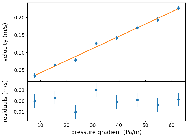
There is no obvious systematic structure in the residuals and the fits look reasonable.

MLEs and errors from multi-parameter model fitting

When using maximum likelihood to fit a model with multiple (\(M\)) parameters \(\pmb{\theta}\), we obtain a vector of 1st order partial derivatives, known as scores:

i.e. \(U(\pmb{\theta})=\nabla L\). In vector calculus we call this vector of 1st order partial derivatives the Jacobian. The MLEs correspond to the vector of parameter values where the scores for each parameter are zero, i.e. \(U(\hat{\pmb{\theta}})= (0,...,0) = \mathbf{0}\).

We saw in the previous episode that the variances of these parameters can be derived from the 2nd order partial derivatives of the log-likelihood. Now let’s look at the case for a function of two parameters, \(\theta\) and \(\phi\). The MLEs are found where:

where we use \(L=L(\phi,\theta)\) for convenience. Note that the maximum corresponds to the same location for both MLEs, so is evaluated at \(\hat{\theta}\) and \(\hat{\phi}\), regardless of which parameter is used for the derivative. Now we expand the log-likelihood function to 2nd order about the maximum (so the first order term vanishes):

The ‘error’ term in the square brackets is the equivalent for 2-parameters to the 2nd order term for one parameter which we saw in the previous episode. This term may be re-written using a matrix equation:

where \(A = \frac{\partial^{2}L}{\partial\theta^{2}}\bigg\rvert_{\hat{\theta},\hat{\phi}}\), \(B = \frac{\partial^{2}L}{\partial\phi^{2}}\bigg\rvert_{\hat{\theta},\hat{\phi}}\) and \(C=\frac{\partial^{2}L}{\partial\theta \partial\phi}\bigg\rvert_{\hat{\theta},\hat{\phi}}\). Since \(L(\hat{\theta},\hat{\phi})\) is a maximum, we require that \(A<0\), \(B<0\) and \(AB>C^{2}\).

This approach can also be applied to models with \(M\) parameters, in which case the resulting matrix of 2nd order partial derivatives is \(M\times M\). In vector calculus terms, this matrix of 2nd order partial derivatives is known as the Hessian. As could be guessed by analogy with the result for a single parameter in the previous episode, we can directly obtain estimates of the variance of the MLEs by taking the negative inverse matrix of the Hessian of our log-likelihood evaluated at the MLEs. In fact, this procedure gives us the covariance matrix for the MLEs. For our 2-parameter case this is:

The diagonal terms of the covariance matrix give the marginalised variances of the parameters, so that in the 2-parameter case, the 1-\(\sigma\) errors on the parameters (assuming the normal approximation, i.e. normally distributed likelihood about the maximum) are given by:

The off-diagonal term is the covariance of the errors between the two parameters. If it is non-zero, then the errors are correlated, e.g. a deviation of the MLE from the true value of one parameter causes a correlated deviation of the MLE of the other parameter from its true value. If the covariance is zero (or negligible compared to the product of the parameter errors), the errors on each parameter reduce to the same form as the single-parameter errors described in the previous episode, i.e.:

Errors from the BFGS optimisation method

The BFGS optimisation method returns the covariance matrix as one of its outputs, so that error estimates on the MLEs can be obtained directly. We currently recommend using the legacy function fmin_bfgs for this approach, because the covariance output from the minimize function’s BFGS method produces results that are at times inconsistent with other, reliable methods to estimate errors. The functionality of fmin_bfgs is somewhat different from minimize as the outputs should be defined separately, rather than as columns in a single structured array.

# Define starting values
p0 = [0.01, 0.003]

# Call fmin_bfgs. To access anything other than the MLEs we need to set full_output=True and 
# read to a large set of output variables. The documentation explains what these are.
ml_pars, ml_funcval, ml_grad, ml_covar, func_calls, grad_calls, warnflag = \
spopt.fmin_bfgs(LogLikelihood, parm, args=(lin_model, xval, yval, dy), full_output=True)

# The MLE variances are given by the diagonals of the covariance matrix:
err = np.sqrt(np.diag(ml_covar))
print("The covariance matrix is:",ml_covar)
print("a = " + str(ml_pars[0]) + " +/- " + str(err[0]))
print("b = " + str(ml_pars[1]) + " +/- " + str(err[1]))
print("Maximum log-likelihood = " + str(-1.0*ml_funcval))

Warning: Desired error not necessarily achieved due to precision loss.
         Current function value: 10.349380
         Iterations: 2
         Function evaluations: 92
         Gradient evaluations: 27
The covariance matrix is: [[ 2.40822114e-05 -5.43686422e-07]
 [-5.43686422e-07  1.54592084e-08]]
a = 0.00752124471628861 +/- 0.004907362976432289
b = 0.0034704797356526714 +/- 0.0001243350648658209
Maximum log-likelihood = -10.349380065702023

We get a warning here but the fit results are consistent with our earlier Nelder-Mead fit, so we are not concerned about the loss of precision. Now that we have the parameters and estimates of their errors, we can report them. A good rule of thumb is to report values to whatever precision gives the errors to two significant figures. For example, here we would state:

\(a = 0.0075 \pm 0.0049\) and \(b = 0.00347 \pm 0.00012\)

or, using scientific notation and correct units:

\(a = (7.5 \pm 4.9)\times 10^{-3}\) m/s and \(b = (3.47\pm 0.12)\times 10^{-3}\) m\(^{2}\)/s/Pa

Weighted least squares

Let’s consider the case where the data values \(y_{i}\) are drawn from a normal distribution about the expectation value given by the model, i.e. we can define the mean and variance of the distribution for a particular measurement as:

and the standard deviation \(\sigma_{i}\) is given by the error on the data value. Note that this situation is not the same as in the normal approximation discussed above, since here it is the data which are normally distributed, not the likelihood function.

The likelihood function for the data points is:

and the log-likelihood is:

Note that the first term on the RHS is a constant defined only by the errors on the data, while the second term is the sum of squared residuals of the data relative to the model, normalised by the squared error of the data. This is something we can easily calculate without reference to probability distributions! We therefore define a new statistic \(X^{2}(\pmb{\theta})\):

This statistic is often called the chi-squared (\(\chi^{2}\)) statistic, and the method of maximum likelihood fitting which uses it is formally called weighted least squares but informally known as ‘chi-squared fitting’ or ‘chi-squared minimisation’. The name comes from the fact that, where the model is a correct description of the data, the observed \(X^{2}\) is drawn from a chi-squared distribution. Minimising \(X^{2}\) is equivalent to maximising \(L(\pmb{\theta})\) or \(l(\pmb{\theta})\). In the case where the error is identical for all data points, minimising \(X^{2}\) is equivalent to minimising the sum of squared residuals in linear regression.

The chi-squared distribution

Consider a set of independent variates drawn from a standard normal distribution, \(Z\sim N(0,1)\): \(Z_{1}, Z_{2},...,Z_{n}\).

We can form a new variate by squaring and summing these variates: \(X=\sum\limits_{i=1}^{n} Z_{i}^{2}\)

The resulting variate \(X\) is drawn from a \(\chi^{2}\) (chi-squared) distribution:

\[p(x\vert \nu) = \frac{(1/2)^{\nu/2}}{\Gamma(\nu/2)}x^{\frac{\nu}{2}-1}e^{-x/2}\]

where \(\nu\) is the distribution shape parameter known as the degrees of freedom, as it corresponds to the number of standard normal variates which are squared and summed to produce the distribution. \(\Gamma\) is the Gamma function. Note that for integers \(\Gamma(n)=(n-1)!\) and for half integers \(\Gamma(n+\frac{1}{2})=\frac{(2n)!}{4^{n}n!} \sqrt{\pi}\). Therefore, for \(\nu=1\), \(p(x)=\frac{1}{\sqrt{2\pi}}x^{-1/2}e^{-x/2}\). For \(\nu=2\) the distribution is a simple exponential: \(p(x)=\frac{1}{2} e^{-x/2}\). Since the chi-squared distribution is produced by sums of \(\nu\) random variates, the central limit theorem applies and for large \(\nu\), the distribution approaches a normal distribution.

A variate \(X\) which is drawn from chi-squared distribution, is denoted \(X\sim \chi^{2}_{\nu}\) where the subscript \(\nu\) is given as an integer denoting the degrees of freedom. Variates distributed as \(\chi^{2}_{\nu}\) have expectation \(E[X]=\nu\) and variance \(V[X]=2\nu\).

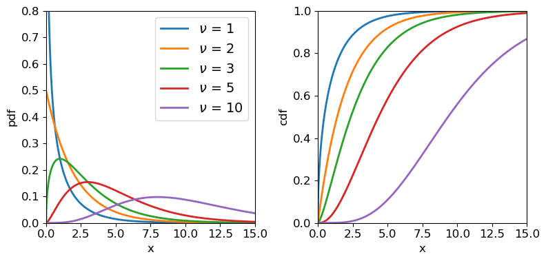
Chi-squared distributions for different degrees of freedom.

Weighted least squares in Python with curve_fit

For completeness, and because it will be useful later on, we will first define a function for calculating the chi-squared statistic:

def ChiSq(parm, model, xval, yval, dy):
    '''Calculates the chi-squared statistic for the input data and model
    Inputs: input parameters, model function name, x and y values and y-errors
    Outputs: chi-squared statistic'''
    
    ymod = model(xval, parm)
    return np.sum(((yval-ymod)/dy)**2)

We already saw how to use Scipy’s curve_fit function to carry out a linear regression fit with error bars on \(y\) values not included. The curve_fit routine uses non-linear least-squares to fit a function to data (i.e. it is not restricted to linear least-square fitting) and if the error bars are provided it will carry out a weighted-least-squares fit, which is what we need to obtain a goodness-of-fit (see below). As well as returning the MLEs, curve_fit also returns the covariance matrix evaluated at the minimum chi-squared, which allows errors on the MLEs to be estimated.

An important difference between curve_fit and the other minimisation approaches discussed above, is that curve_fit implicitly calculates the weighted-least squares from the given model, data and errors. I.e. we do not provide our ChiSq function given above, only our model function (which also needs a subtle change in inputs, see below). Note that the model parameters need to be unpacked for curve_fit to work (input parameters given by *parm instead of parm in the function definition arguments). The curve_fit function does not return the function value (i.e. the minimum chi-squared) as a default, so we need to use our own function to calculate this.

## We define a new model function here since curve_fit requires parameters to be unpacked 
## (* prefix in front of parm to unpack the values in the list)
def lin_cfmodel(value, *parm): 
    '''Linear model suitable for input into curve_fit'''
    return parm[0] + parm[1]*value

p0 = [0.01, 0.003]  # Define starting values
ml_cfpars, ml_cfcovar = spopt.curve_fit(lin_cfmodel, xval, yval, p0, sigma=dy, bounds=([0.0,0.0],[np.inf,np.inf]))
err = np.sqrt(np.diag(ml_cfcovar))
print("The covariance matrix is:",ml_cfcovar)
print("a = " + str(ml_cfpars[0]) + " +/- " + str(err[0]))
print("b = " + str(ml_cfpars[1]) + " +/- " + str(err[1]))

## curve_fit does not return the minimum chi-squared so we must calculate that ourselves for the MLEs
## obtained by the fit, e.g. using our original ChiSq function 
minchisq = ChiSq(ml_cfpars,lin_model,xval,yval,dy)
print("Minimum Chi-squared = " + str(minchisq) + " for " + str(len(xval)-len(p0)) + " d.o.f.")

The covariance matrix is: [[ 2.40651273e-05 -5.43300727e-07]
 [-5.43300727e-07  1.54482415e-08]]
a = 0.0075205140571564764 +/- 0.004905622007734697
b = 0.0034705036788374023 +/- 0.00012429095494525993
Minimum Chi-squared = 5.995743560544769 for 6 d.o.f.

Comparison with our earlier fit using a normal likelihood function and fmin_bfgs shows that the MLEs, covariance and error values are very similar. This is not surprising since chi-squared minimisation and maximum likelihood for normal likelihood functions are mathematically equivalent.

Goodness of fit

An important aspect of weighted least squares fitting is that a significance test, the chi-squared test can be applied to check whether the minimum \(X^{2}\) statistic obtained from the fit is consistent with the model being a good fit to the data. In this context, the test is often called a goodness of fit test and the \(p\)-value which results is called the goodness of fit. The goodness of fit test checks the hypothesis that the model can explain the data. If it can, the data should be normally distributed around the model and the sum of squared, weighted data\(-\)model residuals should follow a \(\chi^{2}\) distribution with \(\nu\) degrees of freedom. Here \(\nu=n-m\), where \(n\) is the number of data points and \(m\) is the number of free parameters in the model (i.e. the parameters left free to vary so that MLEs were determined).

It’s important to remember that the chi-squared statistic can only be positive-valued, and the chi-squared test is single-tailed, i.e. we are only looking for deviations with large chi-squared compared to what we expect, since that corresponds to large residuals, i.e. a bad fit. Small chi-squared statistics can arise by chance, but if it is so small that it is unlikely to happen by chance (i.e. the corresponding cdf value is very small), it suggests that the error bars used to weight the squared residuals are too large, i.e. the errors on the data are overestimated. Alternatively a small chi-squared compared to the degrees of freedom could indicate that the model is being ‘over-fitted’, e.g. it is more complex than is required by the data, so that the model is effectively fitting the noise in the data rather than real features.

Sometimes you will see the ‘reduced chi-squared’ discussed. This is the ratio \(X^2/\nu\), written as \(\chi^{2}/\nu\) and also (confusingly) as \(\chi^{2}_{\nu}\). Since the expectation of the chi-squared distribution is \(E[X]=\nu\), a rule of thumb is that \(\chi^{2}/\nu \simeq 1\) corresponds to a good fit, while \(\chi^{2}/\nu\) greater than 1 are bad fits and values significantly smaller than 1 correspond to over-fitting or overestimated errors on data. It’s important to always bear in mind however that the width of the \(\chi^{2}\) distribution scales as \(\sim 1/\sqrt{\nu}\), so even small deviations from \(\chi^{2}/\nu = 1\) can be significant for larger numbers of data-points being fitted, while large \(\chi^{2}/\nu\) may arise by chance for small numbers of data-points. For a formal estimate of goodness of fit, you should determine a \(p\)-value calculated from the \(\chi^{2}\) distribution corresponding to \(\nu\).

As an example, let’s calculate the goodness of fit for our fit to the Reynolds data:

# The chisq distribution in scipy.stats is chi2
print("The goodness of fit of the linear model is: " + str(sps.chi2.sf(minchisq, df=dof)))

The goodness of fit of the linear model is: 0.4236670604077928

Our \(p\)-value (goodness of fit) is 0.42, indicating that the data are consistent with being normally distributed around the model, according to the size of the data errors. I.e., the fit is good.

Key Points