Significance tests: the t-test - comparing means when population variance is unknown

Overview

Teaching: 30 min
Exercises: 30 min

Questions

• How do I compare a sample mean with an expected value, when I don’t know the true variance that the data are sampled from?

• How do I compare two sample means, when neither the true mean nor variance that the data are sampled from are known?

Objectives

• Learn how to compare normally distributed sample means with an expected value, or two sample means with each other, when only the sample variance is known.

In this episode we will be using numpy, as well as matplotlib’s plotting library. Scipy contains an extensive range of distributions in its ‘scipy.stats’ module, so we will also need to import it. Remember: scipy modules should be installed separately as required - they cannot be called if only scipy is imported.

import numpy as np
import matplotlib.pyplot as plt
import scipy.stats as sps

Comparing the sample mean with a population with known mean but unknown variance

Now let’s return to the speed-of-light data, where we want to compare our data to the known mean of the speed of light in air. Here we have a problem because the speed of light data is drawn from a population with an unknown variance, since it is due to the experimental statistical error which (without extremely careful modelling of the experiment) can only be determined from the data itself.

Therefore we must replace \(\sigma\) in the \(z\)-statistic calculation \(Z = (\bar{x}-\mu)/(\sigma/\sqrt{n})\) with the sample standard deviation \(s_{x}\), to obtain a new test statistic, the \(t\)-statistic :

Unlike the normally distributed \(z\)-statistic, under certain assumptions the \(t\)-statistic can be shown to follow a different distribution, the \(t\)-distribution. The assumptions are:

• The sample mean is normally distributed. This means that either the data are normally distributed, or that the sample mean is normally distributed following the central limit theorem.
• The sample variance follows a scaled chi-squared distribution. We will discuss the chi-squared distribution in more detail in a later episode, but we note here that it is the distribution that results from summing squared, normally-distributed variates. For sample variances to follow this distribution, it is usually (but not always) required that the data are normally distributed. The variance of non-normally distributed data often deviates significantly from a chi-squared distribution. However, for large sample sizes, the sample variance usually has a narrow distribution of values so that the resulting \(t\)-statistic distribution is not distorted too much.

Intuition builder: \(t\)-statistic

We can use the scipy.stats random number generator to see how the distribution of the calculated \(t\)-statistic changes with sample size, and how it compares with the pdfs for the normal and \(t\)-distributions.

First generate many (\(10^{5}\) or more) samples of random variates with sample sizes \(n\) of \(n\) = 4, 16, 64 and 256, calculating and plotting histograms of the \(t\)-statistic for each sample (this can be done quickly using numpy arrays, e.g. see the examples in the central limit theorem episode). For comparison, also plot the histograms of the standard normal pdf and the \(t\)-distribution for \(\nu = n-1\) degrees of freedom.

For your random variates, try using normally distributed variates first, and the uniform variates for comparison (this will show the effects of convergence to a normal distribution from the central limit theorem). Because the t-statistic is calculated from the scaled difference in sample and population means, the distribution parameters won’t matter here. You can use the scipy distribution function defaults if you wish.

Solution part 1

ntrials = 1000000  # Ideally generate at least 100000 samples
# Set the list of sample sizes for the sets of variates generated and used to calculate the t-statistic
nsamp = [4,16,64,256]

# Try with normal and then uniformly distributed variates:
distributions = [sps.norm,sps.uniform]
fig, ax = plt.subplots(2,4, figsize=(10,6))
fig.subplots_adjust(wspace=0.2)
for i in range(2):
    distrib = distributions[i]
    dist = distrib(loc=1,scale=1)
    mu = dist.mean()
    for j in range(4):
        # Generate an array of ntrials samples with size nsamp[j]
        dist_rand = dist.rvs(size=(ntrials,nsamp[j]))
        # Calculate the t-values explicitly to produce an array of t-statistics for all trials
        tvals = (np.mean(dist_rand,axis=1)-mu)/sps.sem(dist_rand,axis=1)
        # Now set up the distribution functions to compare with, first standard normal:
        nd = sps.norm()
        # Next the t-distribution. It has one parameter, the degrees of freedom (df) = sample size - 1  
        td = sps.t(df=nsamp[j]-1)
        plot_range = (-4,4)
        # We are first comparing the histograms:
        dens, edges, patches = ax[i,j].hist(tvals, bins=50, range=plot_range, density=True, alpha=0.3)
        # To get the pdfs in the same bins as the histogram, we calculate the differences in cdfs at the bin
        # edges and normalise them by the bin widths.
        norm_pdf = (nd.cdf(edges[1:])-nd.cdf(edges[:-1]))/np.diff(edges)
        t_pdf = (td.cdf(edges[1:])-td.cdf(edges[:-1]))/np.diff(edges)
        # We can now plot the pdfs as pre-calculated histograms using the trick we learned in Episode 1
        ax[i,j].hist((edges[1:]+edges[:-1])/2,bins=edges,weights=norm_pdf,density=False,
                     histtype='step',linewidth=2,color='orange')
        ax[i,j].hist((edges[1:]+edges[:-1])/2,bins=edges,weights=t_pdf,density=False,
                     histtype='step',linewidth=2,color='green')
        if (i == 0):
            ax[i,j].text(0.1,0.93,"Normal",transform=ax[i,j].transAxes)
        else:
            ax[i,j].text(0.1,0.93,"Uniform",transform=ax[i,j].transAxes)
            
        ax[i,j].text(0.1,0.86,"$n=$"+str(nsamp[j]),transform=ax[i,j].transAxes)
        xticks = np.arange(-4,4.1,1)
        ax[i,j].set_xticks(xticks)
        if j == 0:
            ax[i,j].set_ylabel('prob. density')
        if i == 1:
            ax[i,j].set_xlabel("t")
plt.show()

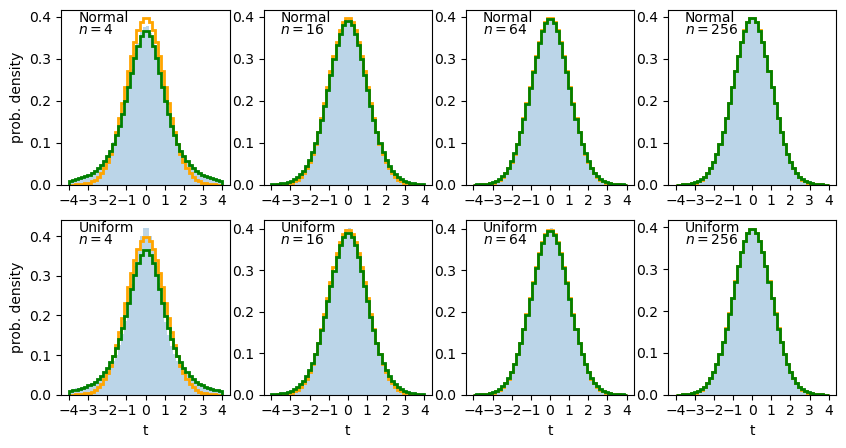
The solid histogram shows the distribution of sample t-statistics for normal (top row) or uniform (bottom row) random variates of sample size \(n\) while the stepped lines show the pdf histograms for the normal (orange) and \(t\)-distribution (green).

We can see that for small \(n\) the distribution of t-statistics has wide ‘tails’ compared to the normal distribution, which match those seen in the t-distribution. For larger \(n\) the t-distribution and the distribution of sample \(t\)-statistics starts to match the normal distribution in shape. This difference is due to the additional variance added to the distribution by dividing by the square-root of sample variance. Sample variance distributions (and hence, the distribution of sample standard deviations) are wider and more asymmetric for smaller sample sizes.

To show the differences between the distributions, and compare uniform and normal variates, it is useful to plot the ratio of the calculated distribution of sample \(t\)-statistics to the pdfs of the normal and \(t\)-distributions. Adapt the code used to plot the histograms, to show these ratios instead.

Solution part 2

fig, ax = plt.subplots(2,4, figsize=(10,6))
fig.subplots_adjust(wspace=0.2)
for i in range(2):
    distrib = distributions[i]
    dist = distrib(loc=1,scale=1)
    mu = dist.mean()
    for j in range(4):
        # Generate an array of ntrials samples with size nsamp[j]
        dist_rand = dist.rvs(size=(ntrials,nsamp[j]))
        # Calculate the t-values explicitly to produce an array of t-statistics for all trials
        tvals = (np.mean(dist_rand,axis=1)-mu)/sps.sem(dist_rand,axis=1)
        # Now set up the distribution functions to compare with, first standard normal:
        nd = sps.norm()
        # Next the t-distribution. It has one parameter, the degrees of freedom (df) = sample size - 1  
        td = sps.t(df=nsamp[j]-1)
        plot_range = (-4,4)
        # Since we no longer want to plot the histogram itself, we will use the numpy function instead
        dens, edges = np.histogram(tvals, bins=50, range=plot_range, density=True)
        # To get the pdfs in the same bins as the histogram, we calculate the differences in cdfs at the bin
        # edges and normalise them by the bin widths.
        norm_pdf = (nd.cdf(edges[1:])-nd.cdf(edges[:-1]))/np.diff(edges)
        t_pdf = (td.cdf(edges[1:])-td.cdf(edges[:-1]))/np.diff(edges)
        # We can now plot the ratios as pre-calculated histograms using the trick we learned in Episode 1
        ax[i,j].hist((edges[1:]+edges[:-1])/2,bins=edges,weights=dens/norm_pdf,density=False,
                     histtype='step',linewidth=2,color='orange')
        ax[i,j].hist((edges[1:]+edges[:-1])/2,bins=edges,weights=dens/t_pdf,density=False,
                     histtype='step',linewidth=2,color='green')
        if (i == 0):
            ax[i,j].text(0.1,0.93,"Normal",transform=ax[i,j].transAxes)
        else:
            ax[i,j].text(0.1,0.93,"Uniform",transform=ax[i,j].transAxes)
            
        ax[i,j].text(0.1,0.86,"$n=$"+str(nsamp[j]),transform=ax[i,j].transAxes)
        ax[i,j].set_ylim(0.5,1.5)
        ax[i,j].tick_params(axis='y',labelrotation=90.0,which='both')
        xticks = np.arange(-4,4.1,1)
        ax[i,j].set_xticks(xticks)
        if j == 0:
            ax[i,j].set_ylabel('ratio')
        if i == 1:
            ax[i,j].set_xlabel("t")
plt.show()

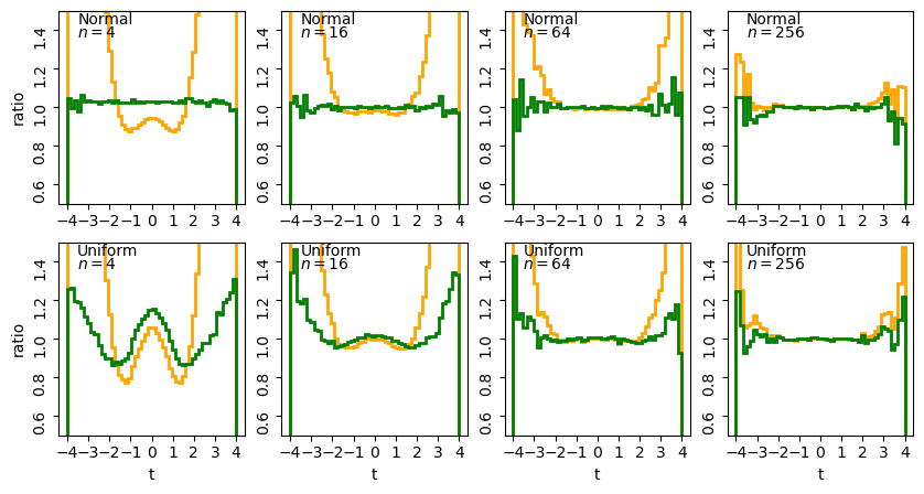
The stepped lines show the ratio of the distribution of sample t-statistics for normal (top row) or uniform (bottom row) random variates of sample size \(n\) relative to the pdf histograms of the normal (orange) and \(t\)-distribution (green).

For small \(n\) we can clearly see the effects of the tails in the ratio to the normal distribution (orange lines) while the ratio for the theoretical \(t\)-distribution (green lines) is much closer to the simulated distribution. It’s interesting to note a few extra points:

• For smaller sample sizes, normally distributed variates show \(t\)-statistics that are consistent with the theoretical distribution. This is because the \(t\)-distribution assumes normally distributed sample means and sample variances which follow a scaled chi-squared distribution, both of which are automatically true for normal variates.
• For uniformly distributed variates, there are strong deviations from the theoretical \(t\)-distribution for small sample sizes, which become smaller (especially in the centre of the distribution) with increasing sample size. These deviations arise firstly because the sample means deviate significantly from the normal distribution for small sample sizes (since, following the central limit theorem, they are further from the limiting normal distribution of a sum of random variates). Secondly, the effects of the deviation from the chi-squared distribution of variance are much stronger for small sample sizes.
• For the large \(n\) the difference between the sample distributions and the theoretical ones (normal or \(t\)-distributions) become indistinguishable for the full range of \(t\). For these samples the theoretical \(t\)-distributions are effectively normally distributed (this is also because of the central limit theorem!) although for uniform variates the distribution of sample \(t\) statistics still does not approach the theoretical distribution exactly in the wings. Scatter in the wings persists even for the normally distributed variates: this is statistical noise due to the small numbers of sample \(t\)-statistics in those bins.

Our overall conclusion is one that applies generally to significance tests: for smaller sample sizes you should always be wary of assigning significances \(>2\) to \(3\) \(\sigma\), unless you are certain that the sample data are also normally distributed.

Probability distributions: the \(t\)-distribution

The \(t\)-distribution is derived based on standard normally distributed variates and depends only on a single parameter, the degrees of freedom \(\nu\). Its pdf and cdf are complicated, involving Gamma and hypergeometric functions, so rather than give the full distribution functions, we will only state the results that for variates \(X\) distributed as a \(t\)-distribution (i.e. \(X\sim t(\nu)\)):

\(E[X] = 0\) for \(\nu > 1\) (otherwise \(E[X]\) is undefined)

\(V[X] = \frac{\nu}{\nu-2}\) for \(\nu > 2\), \(\infty\) for \(1\lt \nu \leq 2\), otherwise undefined.

The distribution in scipy is given by the function scipy.stats.t, which we can use to plot the pdfs and cdfs for different \(\nu\):

nu_list = [1, 2, 5, 10, 100]
fig, (ax1, ax2) = plt.subplots(1,2, figsize=(9,4))
# change the separation between the sub-plots:
fig.subplots_adjust(wspace=0.3)
x = np.arange(-4, 4, 0.01)
for nu in nu_list:
    td = sps.t(df=nu)
    ax1.plot(x, td.pdf(x), lw=2, label=r'$\nu=$'+str(nu))
    ax2.plot(x, td.cdf(x), lw=2, label=r'$\nu=$'+str(nu))
for ax in (ax1,ax2):
    ax.tick_params(labelsize=12)
    ax.set_xlabel("t", fontsize=12)
    ax.tick_params(axis='x', labelsize=12)
    ax.tick_params(axis='y', labelsize=12)
    ax.legend(fontsize=10, loc=2)
ax1.set_ylabel("probability density", fontsize=12)
ax2.set_ylabel("probability", fontsize=12)
plt.show()

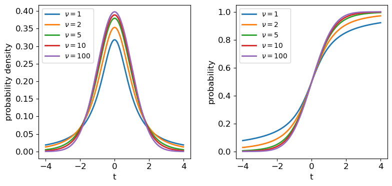
The tails of the \(t\)-distribution are the most prominent for small \(\nu\), but rapidly decrease in strength for larger \(\nu\) as the distribution approaches a standard normal in the limit \(\nu \rightarrow \infty\).

The one-sample \(t\)-test

Finally we are ready to use the \(t\)-statistic to calculate the significance of the difference of our speed-of-light sample mean from the known value, using a test called the one-sample \(t\)-test, or often Students one-sample \(t\)-test, after the pseudonym of the test’s inventor, William Sealy Gossett (Gossett worked as a statistician for the Guiness brewery, who required their employees to publish their research under a pseudonym).

Let’s write down our null hypothesis, again highlighting the statistical (red) and physical (blue) model components:

The samples of speed-of-light measurements are independent variates drawn from a distribution with (population) mean equal to the known value of the speed of light in air and (population) standard deviation given by the (unknown) statistical error of the experiment.

Here the physical part is very simple, we just assume that since the mean is an unbiased estimator, it must be equal to the ‘true’ value of the speed of light in air (\(c_{\rm air}=703\) km/s). We are also implicitly assuming that there is no systematic error, but that is something our test will check. We put ‘(population)’ in brackets to remind you that these are the distribution values, not the sample statistics, although normally that is a given.

Having defined our hypothesis, we also need to make the assumption that the sample mean is normally distributed (this is likely to be the case for 100 samples - the histograms plotted in Episode 1 do not suggest that the distributions are especially skewed and so their sums should converge quickly to being normal distributed). To fully trust the \(t\)-statistic we also need to assume that our sample variance is distributed as a scaled chi-squared variable (or ideally that the data itself is normally distributed). We cannot be sure of this but must make clear it is one of our assumptions anyway, or we can make no further progress!

Finally, with these assumptions, we can carry out a one-sample \(t\)-test on our complete data set. To do so we could calculate \(T\) for the sample ourselves and use the \(t\) distribution for \(\nu=99\) to determine the two-sided significance (since we don’t expect any bias on either side of the true valur from statistical error). But scipy.stats also has a handy function scipy.stats.ttest_1samp which we can use to quickly get a \(p\)-value. We will use both for demonstration purposes:

# First load in the data again (if you need to)
michelson = np.genfromtxt("michelson.txt",names=True)
run = michelson['Run']
speed = michelson['Speed']
experiment = michelson['Expt']

# Define c_air (remember speed has 299000 km/s subtracted from it!)
c_air = 703

# First calculate T explicitly:
T = (np.mean(speed)-c_air)/sps.sem(speed)
# The degrees of freedom to be used for the t-distribution is n-1
dof = len(speed)-1
# Applying a 2-tailed significance test, the p-value is twice the survival function for the given T:
pval = 2*sps.t.sf(T,df=dof)
print("T is:",T,"giving p =",pval,"for",dof,"degrees of freedom")

# And now the easy way - the ttest_1samp function outputs T and the p-value but not the dof:
T, pval = sps.ttest_1samp(speed,popmean=c_air)
print("T is:",T,"giving p =",pval,"for",len(speed)-1,"degrees of freedom")

T is: 18.908867755499248 giving p = 1.2428269455699714e-34 for 99 degrees of freedom
T is: 18.90886775549925 giving p = 1.2428269455699538e-34 for 99 degrees of freedom

The numbers are identical after some rounding at the highest precisions.

Looking deeper at Michelson’s data

Clearly \(\lvert T \rvert\) is so large that our \(p\)-value is extremely small, and our null hypothesis is falsified, whatever reasonable \(\alpha\) we choose for the required significance!
In practice this means that we should first look again at our secondary assumptions about the distribution of sample mean and variance - is there a problem with using the \(t\)-test itself? We know from our earlier simulations that for large samples (e.g. \(n=64\)) the \(t\)-statistic is distributed close to a \(t\)-distribution even for uniformly distributed data. Our data look closer to being normally distributed than that, so we can be quite confident that there is nothing very unusual about our data that would violate those assumptions.

That leaves us with the remaining possibility that the difference is real and systematic, i.e. the sample is not drawn from a distribution with mean equal to the known value of \(c_{\rm air}\). Intuitively we know it is much more likely that there is a systematic error in the experimental measurements than a change in the speed of light itself! (We can put this on firmer footing when we discuss Bayesian methods later on).

However, we know that Michelson’s data was obtained in 5 separate experiments - if there is a systematic error, it could change between experiments. So let’s now pose a further question: are any of Michelson’s 5 individual experiments consistent with the known value of \(c_{\rm air}\)?

We can first carry out a simple visual check by plotting the mean and standard error for each of Michelson’s 5 experiments:

plt.figure()
for i in range(1,6):
    dspeed = speed[experiment == i]
    plt.errorbar(i,np.mean(dspeed),yerr=sps.sem(dspeed),marker='o',color='blue')
# Plot a horizontal line for the known speed:
plt.axhline(703,linestyle='dotted')
plt.xlabel('Experiment',fontsize=14)
plt.ylabel('Speed - 299000 (km/s)',fontsize=14)
# Specify tickmark locations to restrict to experiment ID
plt.xticks(range(1,6))
# The tick marks are small compared to the plot size, we can change that with this command:
plt.tick_params(axis="both", labelsize=12)
plt.show()

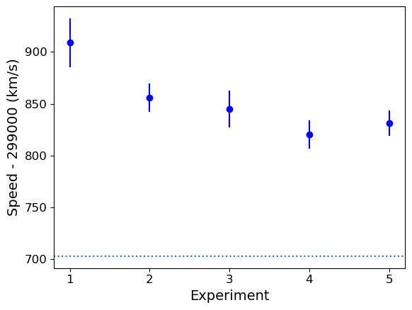
The mean speed for all the experiments are clearly systematically offset w.r.t. the known value of \(c_{\rm air}\) (shown by the dotted line). Given the standard errors for each mean, the offsets appear highly significant in all cases (we could do more one-sample \(t\)-tests but it would be a waste of time, the results are clear enough!). So we can conclude that Michelson’s experiments are all affected by a systematic error that leads the measured speeds to be too high, by between \(\sim 120\) and 200 km/s.

The two-sample \(t\)-test

We could also ask, is there evidence that the systematic error changes between experiments?

To frame this test as a formal null hypothesis we could say:

Two samples (experiments) of speed-of-light measurements are independent variates drawn from the same distribution with (population) mean equal to the known value of the speed of light in air plus an unknown systematic error which is common to both samples and (population) standard deviation given by the (unknown) statistical error of the experiments.

Now things get a little more complicated, because our physical model incorporates the systematic error which is unknown. So to compare the results from two experiments we must deal with unknown mean and variance! Fortunately there are variants of the \(t\)-test which can deal with this situation, called independent two-sample t-tests.

Challenge: comparing Michelson’s experiment means

The independent two-sample t-test uses similar assumptions as the one-sample test to compare the means of two independent samples and determine whether they are drawn from populations with the same mean:

• Both sample means are assumed to be normally distributed.
• Both sample variances are assumed to be drawn from scaled chi-squared distributions. The standard two-sample test further assumes that the two populations being compared have the same population variance, but this assumption is relaxed in Welch’s t-test which allows for comparison of samples drawn from populations with different variance (this situation is expected when comparing measurements of the same physical quantity from experiments with different precisions).

The calculated \(T\)-statistic and degrees of freedom used for the \(t\)-distribution significance test are complicated for these two-sample tests, but we can use scipy.stats.ttest_ind to do the calculation for us.

Experiment 1 shows the largest deviation from the known \(c_{\rm air}\), so we will test whether the data from this experiment is consistent with being drawn from a population with the same mean (i.e. same systematic error) as the other four experiments. Do the following:

1. Look up and read the online documentation for scipy.stats.ttest_ind.
2. Calculate the \(p-value\) for comparing the mean of experiment 1 with those of experiments 2-5 by using both variance assumptions: i.e. first that variances are equal, and then that variances do not have to be equal (Welch’s \(t\)-test).
3. What do you conclude from these significance tests?

Solution

dspeed1 = speed[experiment == 1]
print("Assuming equal population variances:")
for i in range(2,6):
    dspeed0 = speed[experiment == i]
    tstat, pval = sps.ttest_ind(dspeed1,dspeed0,equal_var=True)
    print("Exp. 1 vs. Exp.",i)
    print("T = ",tstat,"and p-value =",pval)
print("\nAllowing different population variances:")
for i in range(2,6):
    dspeed0 = speed[experiment == i]
    tstat, pval = sps.ttest_ind(dspeed1,dspeed0,equal_var=False)
    print("Exp. 1 vs. Exp.",i)
    print("T = ",tstat,"and p-value =",pval)

Assuming equal population variances:
Exp. 1 vs. Exp. 2
T =  1.9515833716400273 and p-value = 0.05838720267301064
Exp. 1 vs. Exp. 3
T =  2.1781204580045963 and p-value = 0.035671254712023606
Exp. 1 vs. Exp. 4
T =  3.2739095648811736 and p-value = 0.0022652870881169095
Exp. 1 vs. Exp. 5
T =  2.9345525158236394 and p-value = 0.005638691935846029

Allowing different population variances:
Exp. 1 vs. Exp. 2
T =  1.9515833716400273 and p-value = 0.06020049646207564
Exp. 1 vs. Exp. 3
T =  2.1781204580045963 and p-value = 0.03615741764675092
Exp. 1 vs. Exp. 4
T =  3.2739095648811736 and p-value = 0.0026588535542915533
Exp. 1 vs. Exp. 5
T =  2.9345525158236394 and p-value = 0.006537756688652282

Relaxing the equal-variance assumption marginally increases the p-values. We can conclude in both cases that the systematic error for Experiment 1 is significantly different to the systematic errors in Experiments 3, 4 and 5 at significances of between 2-3 \(\sigma\).

We need to be cautious however, since we have selected Experiment 1 as being different from the others by using the same data that we are using to compare them, i.e. the result that Experiment 1 is different from the others could be biased by our pre-selection, so that our a posteriori sample selection is not strictly independent of the other experiments!

Furthermore, we have compared this particular extremum in sample mean with multiple other experiments - we might expect some significant differences by chance. So the evidence hints at the possibility that the systematic error changes between experiments, but we should return to these issues later on to be sure.

Challenge: comparing the class height subsamples

Use the two-sample \(t\)-test to compare the means of the two subsamples (denoted 1 and 0) of heights drawn from previous versions of this statistics class (data file class_heights.dat), also clearly stating your null hypothesis and any assumptions, and give your conclusions about the test result.

Solution

Our null hypothesis is that both subsamples are drawn from populations with the same mean (but not necessarily the same variance as this is not specified by the question). To use the two-sample \(t\)-test we must further assume that the sample means are normally distributed and the sample variances are drawn from chi-squared distributions. Since the population distributions for heights are typically normal, both requirements should be satisfied.

# Load the class heights data
class_heights = np.genfromtxt("class_heights.dat")

# Create arrays of the two gender subsamples:
heights0 = class_heights[class_heights[:,1] == 0]
heights1 = class_heights[class_heights[:,1] == 1]

# We need the independent two-sample test allowing for different variances:
tstat, pval = sps.ttest_ind(heights1[:,0],heights0[:,0],equal_var=False)
print("T = ",tstat,"and p-value =",pval)

T =  -4.745757286152359 and p-value = 0.00021922627382520773

The \(p\)-value of 0.0002 gives the probability that if the null hypothesis is true, we would obtain such a large \(\lvert T \rvert\) by chance. We can therefore conclude that the null hypothesis is ruled out, i.e. the subsamples are drawn from populations with different means at more than 3-sigma significance.

Key Points

• A t-statistic can be defined from the sample mean and its standard error, which is distributed following a t-distribution, If the sample mean is normally distributed and sample variance is distributed as a scaled chi-squared distribution.

• The one-sample t-test can be used to compare a sample mean with a population mean when the population variance is unknown, as is often the case with experimental statistical errors.

• The two-sample t-test can be used to compare two sample means, to see if they could be drawn from distributions with the same population mean and either the same or different variances (e.g. to compare measurements of the same quantity obtained with different experiments).

• Caution must be applied when interpreting t-test significances of more than 2 to 3 sigma unless the sample is large or the measurements themselves are known to be normally distributed.