Probability calculus and conditional probability

Overview

Teaching: 40 min
Exercises: 10 min

Questions

• How do we calculate with probabilities, taking account of whether some event is dependent on the occurrence of another?

Objectives

• Learn how to use the probability calculus to calculate the probabilities of events or combinations of events, which may be conditional on each other.

• Learn how conditional probability and the probability calculus can be used to understand multivariate probability distributions.

Sample space and conditional events

Imagine a sample space, \(\Omega\) which contains the set of all possible and mutially exclusive outcomes of some random process (also known as elements or elementary outcomes of the set). In statistical terminology, an event is a set containing one or more outcomes. The event occurs if the outcome of a draw (or sample) of that process is in that set. Events do not have to be mutually exclusive and may also share outcomes, so that events may also be considered as combinations or subsets of other events.

For example, we can denote the sample space of the results (Heads, Tails) of two successive coin flips as \(\Omega = \{HH, HT, TH, TT\}\). Each of the four outcomes of coin flips can be seen as a separate event, but we can also can also consider new events, such as, for example, the event where the first flip is heads \(\{HH, HT\}\), or the event where both flips are the same \(\{HH, TT\}\).

Now consider two events \(A\) and \(B\), whose probability is conditional on one another. I.e. the chance of one event occurring is dependent on whether the other event also occurs. The occurrence of conditional events can be represented by Venn diagrams where the entire area of the diagram represents the sample space of all possible events (i.e. probability \(P(\Omega)=1\)) and the probability of a given event or combination of events is represented by its area on the diagram. The diagram below shows four of the possible combinations of events, where the area highlighted in orange shows the event (or combination) being described in the notation below.

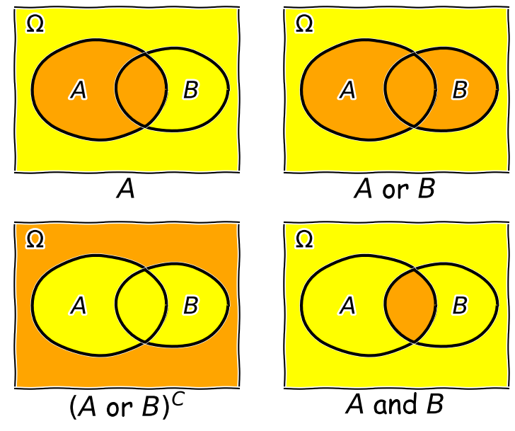
We’ll now decribe these combinations and do the equivalent calculation for the coin flip case where event \(A=\{HH, HT\}\) and event \(B=\{HH, TT\}\) (the probabilities are equal to 0.5 for these two events, so the example diagram is not to scale).

1. Event \(A\) occurs (regardless of whether \(B\) also occurs), with probability \(P(A)\) given by the area of the enclosed shape relative to the total area.
2. Event \((A \mbox{ or } B)\) occurs (in set notation this is the union of sets, \(A \cup B\)). Note that the formal ‘\(\mbox{or}\)’ here is the same as in programming logic, i.e. it corresponds to ‘either or both’ events occurring. The total probability is not \(P(A)+P(B)\) however, because that would double-count the intersecting region. In fact you can see from the diagram that \(P(A \mbox{ or } B) = P(A)+P(B)-P(A \mbox{ and } B)\). Note that if \(P(A \mbox{ or } B) = P(A)+P(B)\) we say that the two events are mutually exclusive (since \(P(A \mbox{ and } B)=0\)).
3. Event \((A \mbox{ or } B)^{C}\) occurs and is the complement of \((A \mbox{ or } B)\) which is everything excluding \((A \mbox{ or } B)\), i.e. \(\mbox{not }(A \mbox{ or } B)\).
4. Event \((A \mbox{ and } B)\) occurs (in set notation this is the intersection of sets, \(A\cap B\)). The probability of \((A \mbox{ and } B)\) corresponds to the area of the overlapping region.

Now in our coin flip example, we know the total sample space is \(\Omega = \{HH, HT, TH, TT\}\) and for a fair coin each of the four outcomes \(X\), has a probability \(P(X)=0.25\). Therefore:

1. \(A\) consists of 2 outcomes, so \(P(A) = 0.5\)
2. \((A \mbox{ or } B)\) consists of 3 outcomes (since \(TH\) is not included), \(P(A \mbox{ or } B) = 0.75\)
3. \((A \mbox{ or } B)^{C}\) corresponds to \(\{TH\}\) only, so \(P(A \mbox{ or } B)^{C}=0.25\)
4. \((A \mbox{ and } B)\) corresponds to the overlap of the two sets, i.e. \(HH\), so \(P(A \mbox{ and } B)=0.25\).

Conditional probability

We can also ask the question, what is the probability that an event \(A\) occurs if we know that the other event \(B\) occurs? We write this as the probability of \(A\) conditional on \(B\), i.e. \(P(A\vert B)\). We often also state this is the ‘probability of A given B’.

To calculate this, we can see from the Venn diagram that if \(B\) occurs (i.e. we now have \(P(B)=1\)), the probability of \(A\) also occurring is equal to the fraction of the area of \(B\) covered by \(A\). I.e. in the case where outcomes have equal probability, it is the fraction of outcomes in set \(B\) which are also contained in set \(A\).

This gives us the equation for conditional probability:

So, for our coin flip example, \(P(A\vert B) = 0.25/0.5 = 0.5\). This makes sense because only one of the two outcomes in \(B\) (\(HH\)) is contained in \(A\).

In our simple coin flip example, the sets \(A\) and \(B\) contain an equal number of equal-probability outcomes, and the symmetry of the situation means that \(P(B\vert A)=P(A\vert B)\). However, this is not normally the case.

For example, consider the set \(A\) of people taking this class, and the set of all students \(B\). Clearly the probability of someone being a student, given that they are taking this class, is very high, but the probability of someone taking this class, given that they are a student, is not. In general \(P(B\vert A)\neq P(A\vert B)\).

Rules of probability calculus

We can now write down the rules of probability calculus and their extensions:

• The convexity rule sets some defining limits: \(0 \leq P(A\vert B) \leq 1 \mbox{ and } P(A\vert A)=1\)
• The addition rule: \(P(A \mbox{ or } B) = P(A)+P(B)-P(A \mbox{ and } B)\)
• The multiplication rule is derived from the equation for conditional probability: \(P(A \mbox{ and } B) = P(A\vert B) P(B)\)

Note that events \(A\) and \(B\) are independent if \(P(A\vert B) = P(A) \Rightarrow P(A \mbox{ and } B) = P(A)P(B)\). The latter equation is the one for calculating combined probabilities of events that many people are familiar with, but it only holds if the events are independent!

We can also ‘extend the conversation’ to consider the probability of \(B\) in terms of probabilities with \(A\):

\[\begin{align} P(B) & = P\left((B \mbox{ and } A) \mbox{ or } (B \mbox{ and } A^{C})\right) \\ & = P(B \mbox{ and } A) + P(B \mbox{ and } A^{C}) \\ & = P(B\vert A)P(A)+P(B\vert A^{C})P(A^{C}) \end{align}\]

The 2nd line comes from applying the addition rule and because the events \((B \mbox{ and } A)\) and \((B \mbox{ and } A^{C})\) are mutually exclusive. The final result then follows from applying the multiplication rule.

Finally we can use the ‘extension of the conversation’ rule to derive the law of total probability. Consider a set of all possible mutually exclusive events \(\Omega = \{A_{1},A_{2},...A_{n}\}\), we can start with the first two steps of the extension to the conversion, then express the results using sums of probabilities:

\[P(B) = P(B \mbox{ and } \Omega) = P(B \mbox{ and } A_{1}) + P(B \mbox{ and } A_{2})+...P(B \mbox{ and } A_{n})\] \[= \sum\limits_{i=1}^{n} P(B \mbox{ and } A_{i})\] \[= \sum\limits_{i=1}^{n} P(B\vert A_{i}) P(A_{i})\]

This summation to eliminate the conditional terms is called marginalisation. We can say that we obtain the marginal distribution of \(B\) by marginalising over \(A\) (\(A\) is ‘marginalised out’).

Challenge

We previously discussed the hypothetical detection problem of looking for radio counterparts of binary neutron star mergers that are detected via gravitational wave events. Assume that there are three types of binary merger: binary neutron stars (\(NN\)), binary black holes (\(BB\)) and neutron-star-black-hole binaries (\(NB\)). For a hypothetical gravitational wave detector, the probabilities for a detected event to correspond to \(NN\), \(BB\), \(NB\) are 0.05, 0.75, 0.2 respectively. Radio emission is detected only from mergers involving a neutron star, with probabilities 0.72 and 0.2 respectively.

Assume that you follow up a gravitational wave event with a radio observation, without knowing what type of event you are looking at. Using \(D\) to denote radio detection, express each probability given above as a conditional probability (e.g. \(P(D\vert NN)\)), or otherwise (e.g. \(P(BB)\)). Then use the rules of probability calculus (or their extensions) to calculate the probability that you will detect a radio counterpart.

Solution

We first write down all the probabilities and the terms they correspond to. First the radio detections, which we denote using \(D\):

\(P(D\vert NN) = 0.72\), \(P(D\vert NB) = 0.2\), \(P(D\vert BB) = 0\)

and: \(P(NN)=0.05\), \(P(NB) = 0.2\), \(P(BB)=0.75\)

We need to obtain the probability of a detection, regardless of the type of merger, i.e. we need \(P(D)\). However, since the probabilities of a radio detection are conditional on the merger type, we need to marginalise over the different merger types, i.e.:

\(P(D) = P(D\vert NN)P(NN) + P(D\vert NB)P(NB) + P(D\vert BB)P(BB)\) \(= (0.72\times 0.05) + (0.2\times 0.2) + 0 = 0.076\)

You may be able to do this simple calculation without explicitly using the law of total probability, by using the ‘intuitive’ probability calculation approach that you may have learned in the past. However, learning to write down the probability terms, and use the probability calculus, will help you to think systematically about these kinds of problems, and solve more difficult ones (e.g. using Bayes theorem, which we will come to later).

Multivariate probability distributions

So far we have considered only univariate probability distributions, but now that we have looked at conditional probability we can begin to study multivariate probability distributions. For simplicity we will focus on the bivariate case, with only two variables \(X\) and \(Y\). The joint probability density function of these two variables is defined as:

This function gives the probability density for any given pair of values for \(x\) and \(y\). In general the probability of variates from the distribution \(X\) and \(Y\) having values in some region \(R\) is:

The probability for a given pair of \(x\) and \(y\) is the same whether we consider \(x\) or \(y\) as the conditional variable. We can then write the multiplication rule as:

From this we have the law of total probability:

i.e. we marginalise over \(y\) to find the marginal pdf of \(x\), giving the distribution of \(x\) only.

We can also use the equation for conditional probability to obtain the probability for \(x\) conditional on the variable \(y\) taking on a fixed value (e.g. a drawn variate \(Y\)) equal to \(y_{0}\):

i.e. we can obtain the probability density \(p(y_{0})\) by integrating the joint probability over \(x\).

Key Points

• A sample space contains all possible mutually exclusive outcomes of an experiment or trial.

• Events consist of sets of outcomes which may overlap, leading to conditional dependence of the occurrence of one event on another. The conditional dependence of events can be described graphically using Venn diagrams.

• Two events are independent if their probability does not depend on the occurrence (or not) of the other event. Events are mutually exclusive if the probability of one event is zero given that the other event occurs.

• The probability of an event A occurring, given that B occurs, is in general not equal to the probability of B occurring, given that A occurs.

• Calculations with conditional probabilities can be made using the probability calculus, including the addition rule, multiplication rule and extensions such as the law of total probability.

• Multivariate probability distributions can be understood using the mathematics of conditional probability.